
“A particle (or car, or bicycle) moves on a number line ….”
These questions may give the position equation, the velocity equation or the acceleration equation of something that is moving, along with an initial condition. The questions ask for information about motion of the particle: its direction, when it changes direction, its maximum position in one direction (farthest left or right), its speed, etc.
The particle may be a “particle,” a person, car, a rocket, etc. Particles don’t really move in this way, so the equation or graph should be considered to be a model. The question is a versatile way to test a variety of calculus concepts since the position, velocity, or acceleration may be given as an equation, a graph, or a table; be sure to use examples of all three forms during the review.
Many of the concepts related to motion problems are the same as those related to function and graph analysis (Type 3). Stress the similarities and show students how the same concepts go by different names. For example, finding when a particle is “farthest right” is the same as finding the when a function reaches its “absolute maximum value.” See my post for November 16, 2012 for a list of these corresponding terms.
The position, s(t), is a function of time. The relationships are
- The velocity is the derivative of the position,
. Velocity is has direction (indicated by its sign) and magnitude. Technically, velocity is a vector; the term “vector” will not appear on the AB exam.
- Speed is the absolute value of velocity; it is a number, not a vector. See my post for November 19, 2012.
- Acceleration is the derivative of velocity and the second derivative of position,
. It, too, has direction and magnitude and is a vector.
- Velocity is the antiderivative of the acceleration
- Position is the antiderivative of velocity.
What students should be able to do:
- Understand and use the relationships above.
- Distinguish between position at some time and the total distance traveled during the time period.
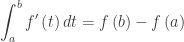
- The total distance traveled is the definite integral of the speed
.
- The net distance traveled, displacement, is the definite integral of the velocity (rate of change):
. Note that “displacement” has not been used preciously on AP exam, but (as per the new Course and Exam Description) may be used now. Be sure your students know this term.
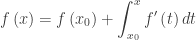
- The final position is the initial position plus the definite integral of the rate of change from x= a to x = t:
Notice that this is an accumulation function equation (Type 1).
- Initial value differential equation problems: given the velocity or acceleration with initial condition(s) find the position or velocity. These are easily handled with the accumulation equation in the bullet above.
- Find the speed at a given time. The speed is the absolute value of the velocity.
- Find average speed, velocity, or acceleration
- Determine if the speed is increasing or decreasing.
- If at some time, the velocity and acceleration have the same sign then the speed is increasing.If they have different signs the speed is decreasing.
- If the velocity graph is moving away from (towards) the t-axis the speed is increasing (decreasing).
- See my post for November 19, 2012.
- Use a difference quotient to approximate derivative.
- Riemann sum approximations.
- Units of measure.
- Interpret meaning of a derivative or a definite integral in context of the problem
Shorter questions on this concept appear in the multiple-choice sections. As always, look over as many questions of this kind from past exams as you can find.
For some previous posts on this subject see November 16, 19, 2012, January 21, 2013. There is also a worksheet on speed here and on the Resources pages (click at the top of this page).
The BC topic of motion in a plane, (Type 8: parametric equations and vectors) will be discussed in a later post.
Next Posts:
Friday March 10: Graph Analysis (Type 3)
Tuesday March 14: Area and Volume (Type 4)
Friday March 17: Table and Riemann sums (Type 5)
Tuesday Match 21: Differential Equations (Type 6)
Friday March 24: Others (Type 7: related rates, implicit differentiation, etc.)
 ,
, is the initial time, and
  is the initial amount. Since this is one of the main interpretations of the definite integral the concept may come up in a variety of situations.
 is the initial time, and


 changes sign.
 . The integral is the difference between whatever f represents at b and what it represents at a. (2009 AB 2 c, AB 3c, 2013 AB3/BC3 c)
 for
for  .
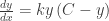
. , where k > 0 is the constant of proportionality, or by
 and
and 
 (D is the constant of integration formally known as “+C.”)
 indicate the location of a horizontal asymptote. There are horizontal asymptotes at y = 0 and y = C.
  , all the factors of the differential equation are positive. This indicates that the function is increasing. Near y = 0 and y = C one factor or the other is small, approaching 0: the graph of the solution (heavy blue line) is leveling off and approaching y = C from below as an asymptote. If the graph is extended into the second quadrant (thin blue line), it approaches the x-axis from above as an asymptote.
 the values of the slope (differential equation) remain positive but decrease indicating that the graph is now increasing and concave down. After this point the two factors of the differential equation switch values; that is, moving the same distance left and right of this point the product will be the same, but the values of each factor will have switched. Thus, the point where
  .
. with sliders for k and C.
 in a volume problem), one point for the integrand, and one point for the numerical answer. An answer alone, with no integral, may not earn any points even if it is correct.
 and
and  . Begin by graphing the functions and finding their points of intersections on your graphing calculator.


