Webinar

Posted on November 28, 2012 by Lin McMullin

You might be interested in this webinar I’m leading

Wednesday December 5, 2012 at 6:30 PM Eastern Standard Time

My Favorite Function: Accumulation and Functions Defined by Integrals

Click here for the recording of this webinar.

Antidifferentiation

Posted on November 28, 2012 by Lin McMullin

Since a lot of classes start integration with antidifferentiation, I’ll discuss that first. If you decide to go with one of the other plans mentioned in my last post, then file this away for later.
____________

The key to finding antiderivatives is pattern recognition.

The simplest integrals are those that follow directly from derivatives such as. Students just need to recognize that the cosine is the derivative of the sine so $\int{\cos \left( x \right)dx}=\sin \left( x \right)+C$ . We wish they were all that simple.

Something like $\int{\tan \left( x \right){{\sec }^{2}}\left( x \right)dx}$ is more complicated. Is the integrand the derivative of $\tfrac{1}{2}{{\tan }^{2}}\left( x \right)$ or of $\tfrac{1}{2}{{\sec }^{2}}\left( x \right)$ ? The answer is yes.

The method called u-substitution helps in identifying the pattern of the integrand. To use this method identify some part of the integrand as a function which you call u and then calculate du and hope that the du is the rest of the integrand.

For $\int{\tan \left( x \right){{\sec }^{2}}\left( x \right)dx}$ you can try u = tan(x) and the du = sec²(x)dx and after making the substitutions:

$\int{\tan \left( x \right){{\sec }^{2}}\left( x \right)dx}=\int{udu}=\tfrac{1}{2}{{u}^{2}}=\tfrac{1}{2}{{\tan }^{2}}\left( x \right)+C$ .

On the other hand we could try u = sec(x) so that du = tan(x)sec(x)dx and

$\int{\tan \left( x \right){{\sec }^{2}}\left( x \right)dx}=\int{\sec (x)\left( \tan (x)\sec (x)dx \right)}$

$=\int{udu}=\tfrac{1}{2}{{u}^{2}}=\tfrac{1}{2}{{\sec }^{2}}\left( x \right)+C*$

(The + C* here not the same as the + C in the expression above: C* = C – ½.)

Either way students need to recognize that part of the integrand is the chain rule contribution to the derivative of the other part of the integrand. The usual three steps to acquire these pattern recognition skills are practice, practice, practice.

Another detail of u-substitution is handling missing constants. For example, $\int{\cos (2x)dx}$ .

Make the substitution u = 2x and then calculate du = 2dx so $dx=\tfrac{1}{2}du$ . Then making these substitutions

$\int{\cos (2x)dx}=\int{\cos \left( u \right)\left( \tfrac{1}{2}du \right)=}\tfrac{1}{2}\int{\cos \left( u \right)du=\tfrac{1}{2}\sin \left( u \right)}$ .

Then back-substituting: $\int{\cos (2x)dx}=\tfrac{1}{2}\sin \left( 2x \right)+C$ .

For simple u-substitutions like this I find it easier to think, and not write, u = 2x so du = 2dx and then write this multiplying by ½ outside the integral sign to account for the extra factor of 2.

$\int{\cos \left( 2x \right)dx=\tfrac{1}{2}\int{\cos \left( 2x \right)\left( 2dx \right)}}=\tfrac{1}{2}\sin \left( 2x \right)+C$ .

This idea only works with missing constants, since only constants can be moved in and out of integrands.

I explain the need for the constant to students by saying that the 2 appears (as if by magic) from the Chain Rule when you differentiate and therefore it must be present to disappear back into the Chain Rule when you antidifferentiate.

Point out to students that integration is very different than differentiation. Differentiation is pretty straightforward; you know what to do when you need to find a derivative. Antidifferentiation is more complicated since recognizing the form or pattern is necessary. The simpler looking integral $\int{\ln \left( x \right)}dx$ is really more difficult than $\int{\tfrac{\ln \left( x \right)}{x}dx}$ .

Finally, if you are teaching antiderivatives before beginning integration, when you get to definite integrals, you will have to remember to show students how to handle the limits of integration by using the same substitution.

For Advanced Placement AB calculus courses these (integrals that follow directly from derivatives and u-substitutions) are the only methods of integration tested. BC students also need to know integration by parts and partial fraction decomposition. I will discuss these later.

Integration Itinerary

Posted on November 26, 2012 by Lin McMullin

Before I write about integration, I’d like to say a few words about the order of topics. Since I assume most of you are AP Calculus teachers, the list of concepts and topics goes something like this:

Area of a region between the graph and the x-axis, which leads to
Riemann sums, which leads to
The definition of the definitive integral.
Numerical integration – left-, right-, upper-, lower-, midpoint sums. The Trapezoidal Rule and Trapezoidal approximations. Integration with technology.
The Fundamental Theorem of Calculus (FTC)
Applications of Integration
Introduction to differential equations.

Your preferred order of topics may be slightly different.

What is missing from this list is antidifferentiation or techniques of integration. There are several places where teachers have placed it with successful results.

1. 1. Many books and therefore many teachers place the topic of antidifferentiation at the very end of the derivative work or the very beginning of the integration. This has the advantage of having your students know how to do at least simple antidifferentiation when they need it right after the FTC. On the other hand, at this point students may not see the need for it and see it as the “game” of reverse differentiation.
  2. A more natural place to tackle it is immediately after the FTC. The advantage here is that now students have a reason to want to antidifferentiate so they can evaluate definite integrals.
  3. Other teachers change the order above slightly and teach applications before the FTC. They set up Riemann sums and definite integrals for the various applications and then have the student evaluate the integrals on their calculators.
    In the usual order listed above each application problem has two parts: the first is to set up the integral and then the antidifferentiation to evaluate it. Often the antidifferentiation is the longer part. By using technology to do the evaluation, students need only concentrate on setting up the correct definite integral and quickly do the evaluation on their calculator.
    Once the students are good at applications they then go on to the FTC and antidifferentiation as separate new topics. While learning antidifferentiation techniques teachers can assign one or two applications each night so students get more practice (spiraling).

I do not advocate one or the other of these approaches. They all have been tried and they all work. I am just pointing out the different ways so you will know that there is a choice. Pick the order you are comfortable with or pick a new order if you want to try something different.

The Derivatives of Exponential Functions

Posted on November 21, 2012 by Lin McMullin

Our problem for today is to differentiate a^x with the (usual) restrictions that a is a positive number and not equal to 1. The reasoning here is very different from that for finding other derivatives and therefore I hope you and your students find it interesting.

The definition of derivative followed by a little algebra gives tells us that

$\displaystyle \frac{d}{dx}{{a}^{x}}=\underset{h\to 0}{\mathop{\lim }}\,\frac{{{a}^{x+h}}-{{a}^{x}}}{h}=\underset{h\to 0}{\mathop{\lim }}\,\frac{{{a}^{x}}{{a}^{h}}-{{a}^{x}}}{h}={{a}^{x}}\underset{h\to 0}{\mathop{\lim }}\,\frac{{{a}^{h}}-1}{h}$ .

Since the limit in the expression above is a number, we observe that the derivative of a^x is proportional to a^x. And also, each value of a gives a different constant. For example if a = 5 then the limit is approximately 1.609438, and so $\displaystyle \frac{d}{{dx}}{{5}^{x}}\approx \left( {1.609438} \right){{5}^{x}}$ .

I determined this by producing a table of values for the expression in the limit near x = 0. You can do the same using a good calculator, computer, or a spreadsheet.

h $\frac{{{5}^{h}}-1}{h}$

-0.00000030 1.60943752

-0.00000020 1.60943765

-0.00000010 1.60943778

0.00000000 undefined

0.00000010 1.60943804

0.00000020 1.60943817

0.00000030 1.60943830

That’s kind of messy and would require us to find this limit for whatever value of a we were using. It turns out that by finding the value of a for which the limit is 1 we can fix this problem. Your students can do this for themselves by changing the value of a in their table until they get the number that gives a limit of 1.

Okay, that’s going to take a while, but may be challenging. The answer turns out to be close to 2.718281828459045…. Below is the table for this number.

h $\frac{{{a}^{h}}-1}{h}$

-0.00000030 0.99999985

-0.00000020 0.99999990

-0.00000010 0.99999995

0.00000000 undefined

0.00000010 1.00000005

0.00000020 1.00000010

0.00000030 1.00000015

Okay, I cheated. The number is, of course, e. Thus,

$\displaystyle \frac{d}{{dx}}{{e}^{x}}={{e}^{x}}\left( {\underset{{h\to 0}}{\mathop{{\lim }}}\,\frac{{{{e}^{h}}-1}}{h}} \right)={{e}^{x}}(1)={{e}^{x}}$ .

The function e^x is its own derivative!

And from this we can find the derivatives of all the other exponential functions. First, we define a new function (well maybe not so new) which is the inverse of the function e^x called ln(x), the natural logarithm of x. (For more on this see Logarithms.) Then a = e^ln(a) and a^x = (e^ln(a))^x = e^(ln(a)x). Then using the Chain Rule, the derivative is

$\frac{d}{dx}{{a}^{x}}={{e}^{(\ln (a))x}}\ln (a)={{\left( {{e}^{\ln (a)}} \right)}^{x}}\ln (a)$

$\frac{d}{dx}{{a}^{x}}={{a}^{x}}\ln \left( a \right)$

Finally, going back to the first table above where a = 5, we find that the limit we found there 1.609438 = ln(5).

For a video on this topic click here.

Revised 8-28-2018, 6-2-2019

Speed

Posted on November 19, 2012 by Lin McMullin

Speed is the absolute value of velocity: speed = $\left| v\left( t \right) \right|$ .

This is the definition of speed, but hardly enough to be sure students know about speed and its relationship to velocity and acceleration.

Velocity is a vector quantity; that is, it has both a direction and a magnitude. The magnitude of velocity vector is the speed. Speed is a non-negative number and has no direction associated with it. Velocity has a magnitude and a direction. Speed has the same value and units as velocity; speed is a number.

The question that seems to trouble students the most is to determine whether the speed is increasing or decreasing. The short answer is

Speed is increasing when the velocity and acceleration have the same sign.

Speed is decreasing when the velocity and acceleration have different signs.

You should demonstrate this in some real context, such as driving a car (see below). Also, you can explain it graphically.

The figure below shows the graph of the velocity $v\left( t \right)$ (blue graph) of a particle moving on the interval $0\le t\le f$ . The red graph is $\left| v\left( t \right) \right|$ , the speed. The sections where $v\left( t \right)<0$ are reflected over the x-axis. (The graphs overlap on [b, d].) It is now quite east to see that the speed is increasing on the intervals [0,a], [b, c] and [d,e].

Another way of approaching the concept is this: the speed is the non-directed length of the vertical segment from the velocity’s graph to the t-axis. Picture the segment shown moving across the graph. When it is getting longer (either above or below the t-axis) the speed increases.

Thinking of the speed as the non-directed distance from the velocity to the axis makes answering the two questions below easy:

1. What are the values of t at which the speed obtains its (local) maximum values? Answer: x = a, c, and e.
2. When do the minimum speeds occur? What are they? Answer: the speed is zero at b and d

Students often benefit from a verbal explanation of all this. Picture a car moving along a road going forwards (in the positive direction) its velocity is positive.

If you step on the gas, acceleration pulls you in the direction you are moving and your speed increases. (v > 0, a > 0, speed increases)
Going too fast is not good, so you put on your brakes, you now accelerate in the opposite direction (decelerate?), but you are still moving forward, but slower. (v > 0, a < 0, speed decreases)
Finally, you stop. Then you shift into reverse and start moving backwards (negative velocity) and you push on the gas to accelerate in the negative direction, so your speed increases. (v < 0, a < 0, speed increases)
Then you put on the breaks (accelerate in the positive direction) and your speed decreases again. (v < 0, a > 0, speed decreases)

Here is an activity that will help your students discover this relationship. Give Part 1 to half the class and Part 2 to the other half. Part 3 (on the back of Part 1 and Part 2) is the same for both groups. – Added 12-19-17

Also see: A Note on Speed for the purely analytic approach.

Update: “A Note on Speed” added 4-21-2018

Motion Problems: Same Thing, Different Context

Posted on November 16, 2012 by Lin McMullin

Calculus is about things that are changing. Certainly, things that move are changing, changing their position, velocity and acceleration. Most calculus textbooks deal with things being dropped or thrown up into the air. This is called uniformly accelerated motion since the acceleration is due to gravity and is constant. While this is a good place to start, the problems are by their nature, somewhat limited. Students often know all about uniformly accelerated motion from their physics class.

The Advanced Placement exams take motion problems to a new level. AB students often encounter particles moving along the x-axis or the y-axis (i.e. on a number line) according to some function that gives the particle’s position, velocity or acceleration. BC students often encounter particles moving around the plane with their coordinates given by parametric equations or its velocity given by a vector. Other times the information is given as a graph or even in a table of the position or velocity. The “particle” may become a car, or a rocket or even chief readers riding bicycles.

While these situations may not be all that “real”, they provide excellent ways to ask both differentiation and integration questions. but be aware that they are not covered that much in some textbooks; supplementing the text may be necessary.

The main derivative ideas are that velocity is the first derivative of the position function, acceleration is the second derivative of the position function and the first derivative of the velocity. Speed is the absolute value of velocity. (There will be more about speed in the next post.) The same techniques used to find the features of a graph can be applied to motion problems to determine things about the moving particle.

So the ideas are not new, but the vocabulary is. The table below gives the terms used with graph analysis and the corresponding terms used in motion problem.

Vocabulary: Working with motion equations (position, velocity, acceleration) you really do all the same things as with regular functions and their derivatives. Help students see that while the vocabulary is different, the concepts are the same.

Function Linear Motion

Value of a function at x position at time t

First derivative velocity

Second derivative acceleration

Increasing moving to the right or up

Decreasing moving to the left or down

Absolute Maximum farthest right

Absolute Minimum farthest left

yʹ = 0 “at rest”

yʹ changes sign object changes direction

Increasing & cc up speed is increasing

Increasing & cc down speed is decreasing

Decreasing & cc up speed is decreasing

Decreasing & cc down speed is increasing

Speed absolute value of velocity

Inverses Graphically and Numerically

Posted on November 14, 2012 by Lin McMullin

In this final post in this series on inverses we consider the graphical and numerical concepts related to the derivative of the inverse and look at an important formula.

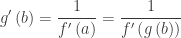
To make the notation a little less messy, let’s let g(x) = f ^-1(x). Then we know that f (g(x))= x. Differentiating this implicitly gives

${f}'\left( g\left( x \right) \right){g}'\left( x \right)=1$
$\displaystyle {g}'\left( x \right)=\frac{1}{{f}'\left( g\left( x \right) \right)}$

Great formula, but one I’ve never been able to memorize and use correctly! It’s my least favorite formula, because I’m never quite sure what to substitute for what.

The graph shows a function and its inverse. It really doesn’t matter which is which, since inverse functions come in pairs: the inverse of the inverse is the original function.

Notice that the graphs are symmetric to y = x. At two points, one of which is the image of the other after reflecting over the line y = x, a tangent segment has been drawn. This segment is the hypotenuse of the “slope triangle” which is also drawn. The ratio of the vertical side of this triangle to the horizontal side is the slope (i.e. the derivative) of the tangent line.

The two triangles are congruent, so that the horizontal side of one triangle is congruent to the vertical side of the other, and vice versa. Thus the slope (the derivative) of the one tangent segment is the reciprocal of the other.

If (a, b) is a point on a function and the derivative at this point is ${f}'\left( a \right)$ , then the point (b, a) is on the function’s inverse and the derivative here is $\displaystyle \frac{1}{{f}'\left( a \right)}$ . This is just what my least favorite formula says: if f ^-1 (x) = g(x), then a = g(b) and $\displaystyle {g}'\left( b \right)=\frac{1}{{f}'\left( a \right)}=\frac{1}{{f}'\left( g\left( b \right) \right)}$ .

What you really need to know is:

At corresponding points on a function and its inverse, the derivatives are reciprocals of each other.

This is what my least favorite formula says.

The AP exams have a clever way of testing this. (The stem may give a few more values to throw you off, or the values may be in a table.)

Given that $f\left( 2 \right)=5\text{ and }{f}'\left( 2 \right)=3$ and g is the inverse of f, Find ${g}'\left( 5 \right)$ .

The solution is reasoned this way: (5, ?) is a point on g. The corresponding point on f is (?, 5) = (2, 5). The derivative of f at this point is 3, therefore the derivative at (5, 2) on g is ${g}'\left( 5 \right)=\tfrac{1}{3}$ .

Easy!

Teaching Calculus

The pleasure lies not in discovering the truth, but in searching for it.

Author Archives: Lin McMullin

Webinar

Antidifferentiation

Integration Itinerary

The Derivatives of Exponential Functions

Speed

Motion Problems: Same Thing, Different Context

Inverses Graphically and Numerically

Share this:

Share this:

Share this:

Share this:

Share this:

Share this:

Share this: