Differential Equations

Posted on January 5, 2015 by Lin McMullin

Differential Equations 1

The next several posts will cover the fundamentals of the topic of differential equations at least as far as is needed for an AP Calculus course. We will begin at the beginning.

What is a differential equation?

A differential equation is an equation with one or more derivatives in it. It may be very simple such as $\displaystyle \frac{dy}{dx}=2x$ , or more complicated such as $\displaystyle \frac{{{d}^{2}}y}{d{{x}^{2}}}+3\frac{dy}{dx}-4y=\cos \left( x \right)$ or even more complicated.

Why do we need differential equations?

It is often not possible to determine directly a regular function that applies to a real situation. However, we may be able to measure how something is changing with respect to time. The change with respect to time is a derivative and gives us a differential equation. Once in college, as you may remember, there are entire courses devoted to using and solving differential equations. Power series (a BC topic) are often used to approximate or find the solution to a differential equation.

What is the solution to a differential equation?

The solution of a differential equation is not a number. For the first equations we will consider the short answer is that a solution is a function that when substituted into the differential equation along with its derivatives produces a true statement (an identity).

As you may suspect differential equations, at least the easy ones, are solved by integrating. Thus the solution of $\frac{dy}{dx}=2x$ first appears to be $y={{x}^{2}}$ . But we quickly realize that $y={{x}^{2}}+17$ and also $y={{x}^{2}}+2\pi$ check when substituted into the given equation. In fact any equation with the form $y={{x}^{2}}+C$ , where C is any constant will check. Because of this we first define the general solution of a differential equation as a function with one or more constants that satisfies the given differential equation.

In order to evaluate the constant(s) we are often given an initial condition. An initial condition is the value of the solution function for a particular value of the independent variable, in other words, a point on the solution’s graph. Once the constant is evaluated, we have what’s called a particular solution.

So if the solution of $\frac{dy}{dx}=2x$ contains the point (4, 7), then the particular solution is $y={{x}^{2}}-9$ . A differential equation with an initial condition is called an initial value problem or an IVP.

How do you solve a differential equation?

There is no one method that will let you solve any differential equation. They are not all as simple as the example above. That’s why entire courses are devoted to solving differential equations. AP Calculus students are expected to know only one of the many methods. (This is because there is only time for the briefest introduction of the topic.) The method is called separation of variables. Not all differential equations can be solved by this method; the second example at the top for example requires a much different approach (that is not tested on the AP calculus exams).

To use the method of separation of variables follow these steps:

(1) by multiplying and dividing rewrite, the equation with the x and dx factors on one side and the y and dy factors on the other side.

(2) Then integrate both sides and

(3) Include a constant of integration.

(4) Use the initial condition to evaluate the constant and

(5) Give the particular solution solved for y.

Example 1: For the very simple example we have been using the work looks like this:

Step 1 Separate the variables: $dy=2xdx$

Steps 2 and 3 Integrate and include the constant of integration. Note that there is a different constant on both sides, but they are immediately combined into one constant that is usually put with the x-terms: $y={{x}^{2}}+C$

Step 4 Use the initial condition to find C: $7={{4}^{2}}+C;\quad C=-9$

Stem 5 Write the solution by solving for y: $y={{x}^{2}}-9$

Example 2: An average difficulty question. Find the particular solution of the differential equation $\displaystyle \frac{dy}{dx}=-\frac{x}{y}$ such that the point (4, –3) lies on the solution.

Step 1: $ydy=-xdx$

Step 2 and 3: $\displaystyle \frac{1}{2}{{y}^{2}}=-\frac{1}{2}{{x}^{2}}+C$ or ${{y}^{2}}=-{{x}^{2}}+C$ . Multiplying by 2 to simplify things, The constant in the second form is not the same as in the first. However, it is just another constant so it is okay to call it C again.

Step 4: ${{(-3)}^{3}}=-{{\left( 4 \right)}^{2}}+C$ so $C=25$

Step 5: ${{y}^{2}}=-{{x}^{2}}+25$ and $y=-\sqrt{25-{{x}^{2}}}$

Since the solution must be a function it is necessary to solve for y by taking the square root of both sides. The negative sign is chosen because the initial condition requires a negative value for y. The solution is a semi-circle, the bottom half of the full circle.

Example 3: A bit more difficult, but the steps are the same. Find the particular solution of the differential equation $\displaystyle \frac{dy}{dx}=\frac{y-1}{{{x}^{2}}}$ with the initial condition $f\left( 2 \right)=0$ . (From the 2008 AB calculus exam question 5c.)

Step 1: $\displaystyle \frac{dy}{y-1}=\frac{dx}{{{x}^{2}}}$

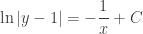
Steps 2 and 3: $\displaystyle \ln \left| y-1 \right|=-\frac{1}{x}+C$

Step 4: When x = 2, y =0 so $\displaystyle \ln \left| 0-1 \right|=-\frac{1}{2}+C;\quad C=\frac{1}{2}$

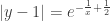
Step 5: Solve for y: $\displaystyle \ln \left| y-1 \right|=-\frac{1}{x}+\frac{1}{2}$

Raise e to the power on each side to remove the natural logarithm. (Students like to call this “E-ing.”)

$\displaystyle {{e}^{\ln }}^{\left| y-1 \right|}={{e}^{-\frac{1}{x}+\frac{1}{2}}}$

$\displaystyle \left| y-1 \right|={{e}^{-\frac{1}{x}+\frac{1}{2}}}$

Near the initial point (2, 0) $\left( y-1 \right)<0$ , so $\left| y-1 \right|=-\left( y-1 \right)=1-y$ , so

$\displaystyle 1-y={{e}^{-\frac{1}{x}+\frac{1}{2}}}$

$\displaystyle y=1-{{e}^{-\frac{1}{x}+\frac{1}{2}}}$

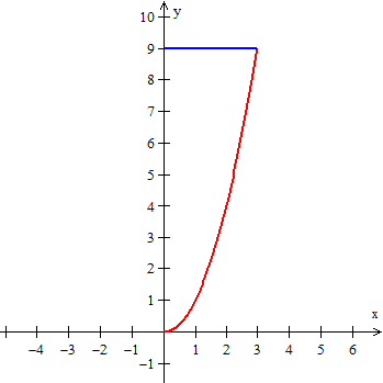
The graph of the solution is the part of the graph shown below for which $x>0$ . See note 2 below:

Two final notes:

The business with the absolute values is important. Students seem to prefer just ignoring the absolute values, but of course you cannot do that. A similar thing occurred in example 2: since you need the square root of one side you must decide, based on the initial condition, whether to use a plus or a minus sign with the radical. Some practice with both these situations is needed.
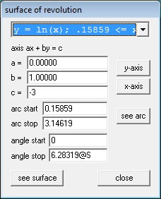
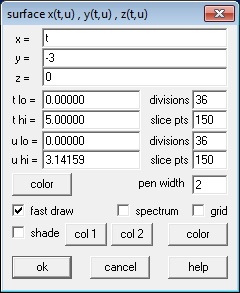
Since $\left( y-1 \right)<0,\quad y<1$ . In order to make this so, $x>0$ . This is the domain of the solution. Technically, the domain of the particular solution of a differential equation must be an open interval that contains the initial condition, and on which the differential equation is true. Practically, this means that the graph must go through the initial condition point but may not cross an asymptote or contain a point where the function is not defined. The solution in the example is undefined at x = 0. It approaches the y-axis as a vertical asymptote from the left and approaches the point (0,1) from the right. AP students were not required to sort all this out, but a simple graph of the solution will show what’s happening. For more on the domain (which is not really tested) click here.
For you techies: The graph was made on an iPad using an app called Good Grapher Pro. This is an excellent grapher for 2D and 2D graphs that zoom easily by pinching the screen (of course).

January

Posted on January 1, 2015 by Lin McMullin

Happy New Year!

The January posts from past years finish the methods of integration thread from December and then go onto applications of integration: area between graphs, volume, and average value of a function. The month ends with a series on accumulation and functions defined by integrals.These run into February, so I’ve included them in the list below.

The most popular post from past Januarys by far is the AP Accumulation Question post. It is in the featured list below along with some others from past Januarys.

Later this month look for a new series of post on differential equations

January 2, 2013 Integration by Parts – 1

January 4, 2013 Integration by Parts – 2

January 7, 2013 Area Between Curves

January 9, 2013 Volume of Solids with Regular Cross-sections

January 11, 2013 Volumes of Revolution

January 14, 2013 Why You Never Need Cylindrical Shells

January 16, 2013 Average Value of a Function

January 19, 2013 Most Triangles are Obtuse! What is the probability that a triangle picked at random will be acute? An average value problem.

January 21, 2103 Accumulation: Need an Amount? Accumulation 1: If you need an amount, look around for a rate to integrate.

January 23, 2013 AP Accumulation Questions Accumulation 2: AP Exam Rate/Accumulation Questions

January 25, 2014 Improper Integrals and Proper Areas

January 26, 2013 Graphing with Accumulation 1 Accumulation 3: Graphing Ideas in Accumulation – Increasing and decreasing

January 28, 2013 Graphing with Accumulation: Accumulation 4: Graphing Ideas in Accumulation – Concavity

January 30, 2013 Stamp Out Slope-intercept Form! Accumulation 5: Lines

February 2, 2013: Accumulation and Differential Equations Accumulation 6: Differential equations

February 4, 2013: Painting a Point Accumulation 7: An application (of paint)

Foreshadowing the FTC

Posted on December 15, 2014 by Lin McMullin

This is an example to help prepare students to tackle the Fundamental Theorem of Calculus (FTC). Use it after the lesson on Riemann sums and the definition of the definite integral, but before the FTC derivation.

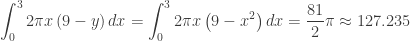
Consider the area, A, between the graph of $f\left( x \right)=\cos \left( x \right)$ and the x-axis on the interval $\left[ 0,\tfrac{\pi }{2} \right]$ . Set up a Riemann sum using the general partition:

$0={{x}_{0}}<{{x}_{1}}<{{x}_{2}}<{{x}_{3}}<\cdots <{{x}_{n-2}}<{{x}_{n-1}}<{{x}_{n}}=\tfrac{\pi }{2}$

$\displaystyle A=\int_{0}^{{\scriptstyle{}^{\pi }\!\!\diagup\!\!{}_{2}\;}}{\cos \left( x \right)dx}=\underset{\Delta x\to 0}{\mathop{\lim }}\,\sum\limits_{i=1}^{n}{\cos \left( {{c}_{i}} \right)\left( {{x}_{i}}-{{x}_{i-1}} \right)}$

Since we can choose the value of ${{c}_{i}}$ any way we want, let’s take the same intervals and use ${{c}_{i}}$ the number guaranteed by the Mean Value Theorem for the function $F\left( x \right)=\sin \left( x \right)$ on the each sub-interval interval. That is, on each sub-interval at $x={{c}_{i}}$

$\left. \frac{d}{dx}\sin \left( x \right) \right|_{x={{c}_{i}}}^{{}}=\cos \left( {{c}_{i}} \right)=\frac{\sin \left( {{x}_{i}} \right)-\sin \left( {{x}_{i-1}} \right)}{\left( {{x}_{i}}-{{x}_{i-1}} \right)}$

Then, substituting into the Riemann sum above

$\displaystyle A=\underset{\Delta x\to 0}{\mathop{\lim }}\,\sum\limits_{i=1}^{n}{\cos \left( {{c}_{i}} \right)\left( {{x}_{i}}-{{x}_{i-1}} \right)}=\underset{\Delta x\to 0}{\mathop{\lim }}\,\sum\limits_{i=1}^{n}{\frac{\sin \left( {{x}_{i}} \right)-\sin \left( {{x}_{i-1}} \right)}{\left( {{x}_{i}}-{{x}_{i-1}} \right)}\left( {{x}_{i}}-{{x}_{i-1}} \right)}$

$\displaystyle A=\underset{\Delta x\to 0}{\mathop{\lim }}\,\sum\limits_{i=1}^{n}{\left( \sin \left( {{x}_{i}} \right)-\sin \left( {{x}_{i-1}} \right) \right)}$

Now writing out the terms we have a telescoping series:

$\displaystyle A=\left( \sin \left( {{x}_{1}} \right)-\sin \left( {{x}_{0}} \right) \right)+\left( \sin \left( {{x}_{2}} \right)-\sin \left( {{x}_{1}} \right) \right)+\left( \sin \left( {{x}_{3}} \right)-\sin \left( {{x}_{2}} \right) \right)+$

$\displaystyle \cdots +\left( \sin \left( {{x}_{n-1}} \right)-\sin \left( {{x}_{n-2}} \right) \right)+\left( \sin \left( {{x}_{n}} \right)-\sin \left( {{x}_{n-1}} \right) \right)$

$\displaystyle A=\sin \left( {{x}_{n}} \right)-\sin \left( {{x}_{0}} \right)$

$\displaystyle A=\sin \left( \tfrac{\pi }{2} \right)-\sin \left( 0 \right)=1$

As you can see, this is really just the derivation of the FTC applied to a particular function. Now the students should have a better idea of what’s going on when you solve the problem in general, i.e. when you prove the FTC.

December

Posted on December 1, 2014 by Lin McMullin

Which are you looking forward to more: winter vacation or teaching Riemann sums and the FTC? Well okay, vacation; me too – except that being retired is like vacation almost every day. Anyway, before vacation or certainly right after comes Riemann sums and the Fundamental Theorem, one of my favorite parts of the curriculum.

This is the list of past posts for December. There are a few new ones in the works for this year. The lead up to integration starts with three activities to get students started on integration ideas: “The Old Pump” , “Flying Into Integrationland.” and “Jobs, Jobs, Jobs.” The next four are the “featured post” below the first post on the home page; they form a series leading up to the Fundamental Theorem of Calculus. (The blog lists them automatically in most-recent-first order so I cannot change the order. Start with “Working Towards Riemann Sums” and read backwards.) Don’t skip the post “More on the FTC.”

Happy Holidays!

December: Introducing Integration, Riemann Sums, the Definite Integral, the Fundamental Theorem of Calculus, properties of integrals

November 30, 2012 The Old Pump

December 3, 2012 Flying In to Integration Land

December 5, 2012 Jobs, Jobs, Jobs

December 7, 2012 Under is a Long Way Down

December 10, 2012 Working Towards Riemann Sums

December 12, 2012 Riemann Sums

December 14, 2012 The Definition of the Definite Integral

December 17, 2012 The Fundamental Theorem of Calculus

December 19, 2012 More about the FTC

December 21, 2012 Properties of Integrals

An extra post more related to derivative applications:December 8, 2012 Inequalities

Visualizing Solid Figures 5

Posted on November 25, 2014 by Lin McMullin

To end this series of posts on visualizing solid figures, we will look at a problem that relates to how volumes of solid figures are formed. It has 5 parts which will be presented first. Then the solution will be given.

Consider the region in the first quadrant bounded by the graphs of the parabola $y={{x}^{2}}$ and the line $y=9$ both for $0\le x\le 3$ .

This region is revolved around the y-axis to form a solid figure.

Use the disk/washer method to find the volume of this figure.
Use the method of cylindrical shells to find the volume of this figure.
Use the disk/washer method to find a number j , such that when x = j the volume of the figure is one-half that of the original figure.
Use the method of cylindrical shells to find a number k , such that when x = k the volume of the figure is one-half that of the original figure.
The answers to parts a) and b) should be the same, but the answers to parts c) and d) are different. Explain why they are different.

Solutions:

1. The volume by the disk/washer method is

$\displaystyle V=\int_{0}^{9}{\pi {{x}^{2}}dy}=\int_{0}^{9}{\pi ydy}=\frac{81}{2}\pi \approx 127.235$

2. The volume by the method of cylindrical shells is

$\displaystyle \int_{0}^{3}{2\pi x\left( 9-y \right)dx}=\int_{0}^{3}{2\pi x\left( 9-{{x}^{2}} \right)dx}=\frac{81}{2}\pi \approx 127.235$

3. The value is be found by solving the equation for j:

$\displaystyle \int_{0}^{{{j}^{2}}}{\pi y\,dy}=\frac{81}{4}\pi$ , so $j\approx 2.52269$

4. The value is be found by solving the equation for k:

$\displaystyle \int_{0}^{k}{2\pi x\left( 9-{{x}^{2}} \right)dx}=\frac{81}{4}\pi$ and $k\approx 1.62359$

5. The reason the values are not the same is this. Think of the revolved parabola as a bowl. If you pour water into the bowl until it is half full, the bowl looks like the figure below. The water is pooled in the bottom of the bowl as you would expect. This is what happens when using the disk/washer method. The washers stack up starting in the bottom of the bowl until it is half full.

On the other hand, the method of cylindrical shells sort of wraps the water in layers (the shells) around the y-axis. Picture the water being sprayed on the y-axes and frozen there. Each new layer (shell) increases the amount and you end up half of the total volume arranged as a cylinder with a rounded (paraboloid shaped) bottom as shown in the figure below. Both bowls contain the same amount of water, arranged differently.

Visualizing Solid Figures 4

Posted on November 22, 2014 by Lin McMullin

Volume by the method of “Cylindrical Shells”

Today I will show you how to visualize the cylindrical shells used in computing the volume using Winplot.

Winplot is a free program. Click here for Winplot and here for Winplot for Macs.

For the example I will use the same situation as in the last post. This was an AP question from 2006 AB1 / BC 1. In part (c) students were asked to find the volume of the solid figure formed when the region between the graphs of y = ln(x) and y = x – 2 is revolved around the y-axis. This can be done by the washer method, but some students use the method of cylindrical shells. We found that the graphs intersect at x = 0.15859 and x = 3.14619.

Begin as before by graphing the two functions and the vertical segment joining them.

In Winplot open a 2D window, click on Equa > 1. Explicit and enter the first equation. Click the “lock interval” box and enter 0.159 for the “low x,” and 3.146 for the “high x,” choose a color and click “ok.”
Repeat this for the second equation.
Then return to Equa > Segment > (x,y) and enter the endpoints of the vertical segment joining the graphs: x1 = B, y1 = ln(B), x2 = B, and y2 = B – 2. Choose a color and click “ok.”
Click Anim > individual > B to open a slider box for B. Type 0.159 and click “set L” and then type 3.146 and click “set R.” Use this slider to move the thin Riemann sum rectangle across the region.

Next draw the 3D graphs:

Click One > Revolve Surface. The equations will appear in the drop-down box at the top of the window. Graphs are revolved one at a time. For the first graph click the “y-axis” button to put the correct values for a, b, and c in the boxes. In the “arc start” box type 0.159 and in the “arc stop” box type 3.146, the ends of the interval. In the “angle stop” box type 2pi@S. (S for surface.) See the figure below. Click “see surface.”

Repeat this by selecting the second function from the drop-down box. Leave all the values the same and click enter. The two surfaces will be graphed in the same color as the corresponding functions in the 2D set up.
Repeat this for the segment, but change the 2p@S in “arc stop” box to 2p@R. (R for Riemann rectangle.) Click “see surface.”
You will need to make one adjustment at this point. In the 3D Inventory list choose the segment and click “edit.” In the box change “low t” to 0 and the “high t” to 1. See the next figure.

In the 3D window, click Anim > Individual and open slider boxes for B, R, and S.
In the B box enter 0.159 and click “set L” and enter 3.146 and click “set R.” These are the endpoints.
In the S box make “set L” = -2pi. “Set R” should already be 2pi. Then type 0 and Enter.
The R box should open with “set L” = 0 and “Set R” = 2pi. no changes are necessary.

Move first the B slider, then the R slider, then the B slider again and finally the S slider to explore the situation.
Type Ctrl+A to show the axes. Use the 4 arrow keys to move the figure around, and the page up and page down keys to zoom in and out.

That should do it.

In the video above you will see

The Riemann rectangle moving in the plane using the B slider.
The Riemann rectangle rotated around the y-axis using the R slider.
The shell moving through the curves using the B slider again.
The two curves rotated part way using the S slider.
The shell moving through the solid using the B slider.

The next and last post in this series will be a question to see if you understand how the washer method and the cylindrical shell method work in a real situation.

Update:One of my favorite post is Difficult Problems and Why We Like Them from June 10, 2013. In it I mention a sculpture called Kryptos located at CIA headquarters in Langley, Virginia. The sculpture contains four enciphered messages. Only three of these have been deciphered since the sculpture was erected in 1990. The sculptor has offered a second clue to the fourth message. I’ve added links story and clues in the original post; see if you can decipher the fourth part.

Visualizing Solid Figures 3

Posted on November 19, 2014 by Lin McMullin

Volume by “Washers”

Today I will show you how to visualize not just the solid figures but the disks and washers used in computing the volume using Winplot. The next post will show how to draw shells.

Winplot is a free program. Click here for Winplot and here for Winplot for Macs.

For the example we’ll use the situations from the 2006 AP calculus exams question AB1 / BC 1. The students were given the region between the graphs of y = ln(x) and y = x -2. In the first part they were asked to find the area of the region. To do that they first had to determine, using their calculator, where the curves intersect. The x-coordinates of the intersections are x = 0.15859 and x = 3.14619.

In part (b) they were asked to find the volume of the solid formed when the region was rotated around the horizontal line y = -3 . The volume is found by using the disk/washer method. Here is how to show the washers using Winplot. This gets a little complicated so I will mark each step with a bullet

Starting in the 2D window, graph the two functions as shown in the previous post.. When entering the equations click the “lock interval” box and enter 0.159 for “low x” and 3.146 for “high x.”
Next we will enter a Riemann sum rectangle which we will be able to move, and, once rotated, will appear as the washer. Go to Equa > Segment > (x,y) and in the box enter the endpoints of the vertical segment between the two graphs in terms of B: x1 = B, y1 = ln(B), x2 = B, and y2 = B – 2. Click “ok.”
Go to the Anim button, choose “B” (Anim > Individual > B).
Enter the left value 0.15859 and click “set L”, and enter 3.14619 and click “set R.” (Remember how to do this, as we will do it again.)
You may now move the “Riemann rectangle” (which, of course, is very thin, approaching 0) across the region.

Next we will produce the 3D images.

As we did in the last post click on One > Revolve surface… Enter the values shown below. (The “arc start” and “arc stop” value are the x-values of the intersection points. Attach an “@S” to the “angle stop” as shown.)

Click “see surface.”
In the 3D window that appears click Anim > S and you will be able to revolve the curve. Make the “set L” value -2pi by typing the value in the box and clicking “set L,” leave “set R” at 2pi. Adjust the value to 0 by typing 0 and “enter.”
Adjust the viewing widow with the 4 arrow keys and the Page Up and Page down keys. Add the axes with Ctrl+A.
Return to the “surface of revolution” window and choose the second function from the drop-down box at the top. not change anything else. Click “see surface” and the second curve will be added to the graph.

Next we graph the “washer:”

In the surface of revolution box, select the segment in the drop-down box at the top change the “angle stop” to 2pi@R. Click “ok.”
Then in the 3D Inventory window for this file select the segment and click “edit.”
Change the “low t” value to 0 and the “high t” value to 1. Change the “u hi” to 2pi@R. Click “ok.” The window should look like the one below.

Finally, in the 3D window:

To show the line y = –3, in the 3D window go to Equa > 2. Parametric and enter the values shown in the box below and click “ok.” A short segment at y = -3 will appear in the 3D window.
In the 3D window go to Anim > Individual and open a slider for “B” and for “R.”
For the “B” slider make “set L” = 0.15859 and the “set R” to 3.14619 (the intersection values).
For the “R” slide make “set L” to 0 and “set R” to 2pi.
Adjust the R and S sliders to 0 and the B slider to its minimum value.
Save everything just to be safe. The extension will be “.wp3.” Later you can open this file from the 3D window, but it will no longer be in touch with the 2D window even if you save that.

That should do it.

Move first the B slider, then the R slider, then the B slider again and finally the S slider to explore the situation.

In the video at the top you will see this example with these things happening in order.

The Riemann rectangle moving in the plane using the B slider
The Riemann rectangle rotated into a washer using the R slider.
The washer moving through the curves using the B slider again.
The two curves rotated part way using the S slider
The washer moving through the solid using the B slider.
The solid rotated with the 4 arrow keys.

The next post will show how to do a similar animation for the cylindrical shell method.

Teaching Calculus

The pleasure lies not in discovering the truth, but in searching for it.

Author Archives: Lin McMullin

Differential Equations

January

Happy New Year!

Foreshadowing the FTC

December

Visualizing Solid Figures 5

Visualizing Solid Figures 4

Visualizing Solid Figures 3

Share this:

Happy New Year!

Share this:

Share this:

Share this:

Share this:

Share this:

Share this: