Determining the Indeterminate 2

Posted on December 6, 2015 by Lin McMullin

The other day someone asked me a question about the implicit relation ${{x}^{3}}-{{y}^{2}}+{{x}^{2}}=0$ . They had been asked to find where the tangent line to this relation is vertical. They began by finding the derivative using implicit differentiation:

$3{{x}^{2}}-2y\frac{dy}{dx}+2x=0$

$\displaystyle \frac{dy}{dx}=\frac{3{{x}^{2}}+2x}{2y}$

The derivative will be undefined when its denominator is zero. Substituting y = 0 this into the original equation gives ${{x}^{3}}-0+{{x}^{2}}=0$ . This is true when x = –1 or when x = 0. They reasoned that there will be a vertical tangent when x = –1 (correct) and when x = 0 (not so much). They quite wisely looked at the graph.

${{x}^{3}}-{{y}^{2}}+{{x}^{2}}=0$

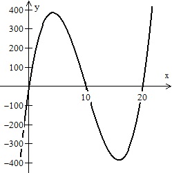
The graph appears to run from the first quadrant, through the origin into the third quadrant, up to the second quadrant with a vertical tangent at x = –1, and then through the origin again and down into the fourth quadrant. It looks like a string looped over itself.

What’s going on at the origin? Where is the vertical tangent at the origin?

The short answer is that vertical tangents occur when the denominator of the derivative is zero and the numerator is not zero. When x = 0 and y = 0 the derivative is an indeterminate form 0/0.

In this kind of situation an indeterminate form does not mean that the expression is infinite, rather it means that some other way must be used to find its value. L’Hôpital’s Rule comes to mind, but the expression you get results in another 0/0 form and is no help (try it!).

My thought was to solve for y and see if that helps:

$y=\pm \sqrt{{{x}^{3}}+{{x}^{2}}}$

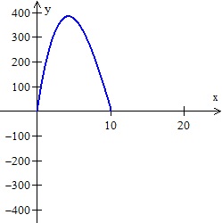
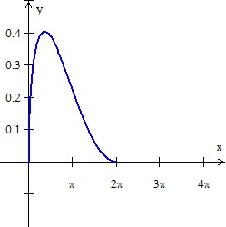
The graph consists of two parts symmetric to the x-axis, in the same way a circle consists of two symmetric parts above and below the x-axis. The figure below shows the top half.

$y=+\sqrt{{{x}^{3}}+{{x}^{2}}}$

So, the graph does not run from the first quadrant to the third; rather, at the origin it “bounces” up into the second quadrant. The lower half is congruent and is the reflection of this graph in the x-axis.

So, what happens at the origin and why?

The derivative of the top half is $\displaystyle \frac{dy}{dx}=\frac{3{{x}^{2}}+2x}{2\sqrt{{{x}^{3}}+{{x}^{2}}}}$ . Notice that this is the same as the implicit derivative above. Now a little simplifying; okay a lot of simplifying – who says simplifying isn’t that big a deal?

$\displaystyle \frac{dy}{dx}=\frac{x\left( 3x+2 \right)}{2\sqrt{{{x}^{2}}\left( x+1 \right)}}=\frac{x\left( 3x+2 \right)}{2\left| x \right|\sqrt{x+1}}=\left\{ \begin{matrix} \frac{3x+2}{2\sqrt{x+1}} & x>0 \\ -\frac{3x+2}{2\sqrt{x+1}} & x<0 \\ \end{matrix} \right.$

Now we see what’s happening. As x approaches zero from the right, the derivative approaches +1, and as x approaches zero from the left, the derivative approaches –1. This agrees with the graph. Since the derivative approaches different values from each side, the derivative does not exist at the origin – this is not the same as being infinite. (For the lower half, the signs of the derivative are reversed, due to the opposite sign of the denominator.)

The tangent lines at the origin are x = 1 on the right, and x = –1 on the left, hardly vertical.

What have we learned?

Indeterminate forms do not necessarily indicate an infinite value. An indeterminate form must be investigated further to see what you can learn about a function, relation, or graph.
Sometimes simplifying, or at least changing the form of an expression, is helpful and therefore necessary.

Extension: Using a graphing utility that allows sliders (Winplot, GeoGebra, Desmos, etc) enter $A{{x}^{3}}-B{{y}^{2}}+C{{x}^{2}}=0$ and explore the effects of the parameters on the graph.

_________________________

The Man Who Tried to Redeem the World with Logic

WALTER PITTS (1923-1969): Walter Pitts’ life passed from homeless runaway, to MIT neuroscience pioneer, to withdrawn alcoholic. (Estate of Francis Bello / Science Source)

I ran across this article that you might find interesting. It is about Walter Pitts one of the twentieth century’s most important mathematicians we, or at least I, have never heard of. It is from the February 5, 2015 of the science magazine Nautilus

December 2015

Posted on December 1, 2015 by Lin McMullin

Here are the past posts for December. The topics are those leading to integration and the Fundamental Theorem of Calculus. The four featured post below are the most popular December posts from past years.

I hope you all have a happy holiday season as you get ready for the New Year.

November 18, 2012 Antidifferentiation

November 26, 2012 Integration Itinerary

November 30, 2012 The Old Pump

December 3, 2012 Flying In to Integration Land

December 5, 2012 Jobs, Jobs, Jobs

December 7, 2012 Under is a Long Way Down

December 8, 2012 Inequalities

December 10, 2012 Working Towards Riemann Sums

December 12, 2012 Riemann Sums

December 14, 2012 The Definition of the Definite Integral

December 17, 2012 The Fundamental Theorem of Calculus

December 19, 2012 More about the FTC

December 21, 2012 Properties of Integrals

November 2015

Posted on October 31, 2015 by Lin McMullin

Here is the list of “November Topics,” that is what AP classes usually consider from mid-November into December. There has been a lot of discussion about inverses this month at the AP Calculus Community. While not the most read on this blog, the series on inverses may be helpful in considering all the ins and outs of inverses.

The four featured posts on the first page are the most popular from this month. Speed with 3563 hits this year and 6157 hits since it first appear is one of the most popular overall. “Open or Closed?” is another poplar post.

Thinking ahead into December, the first posts on integration are here and will continue into December. (As I’ve mentioned I try to post a few weeks ahead of where most people are now, so you have some time to read and plan.)

October 13, 2014 Extremes without Calculus

November 2, 2012 Open or Closed?

November 5, 2012 Inverses

November 7, 2012 Writing Inverses

November 9, 2012 The Range of the Inverse

November 12, 2012 The Calculus of Inverses

November 14, 2012 Inverses Graphically and Numerically

November 16, 2012 Motion Problems: Same Thing, Different Context.

November 19, 2012 Speed

April 17, 2013 The Ubiquitous Particle Motion Question

September 16, 2014 Matching Motion

November 21, 2012 Derivatives of Exponential Functions

November 26, 2012 Integration Itinerary

November 18, 2012 Antidifferentiation

November 30, 2012 The Old Pump

Curves with Extrema?

Posted on October 19, 2015 by Lin McMullin

We spend a lot of time in calculus studying curves. We look for maximums, minimums, asymptotes, end behavior, and on and on, but what about in “real life”?

For some time, I’ve been trying to find a real situation determined or modeled by a non-trigonometric curve with more than one extreme value. I’ve not been very successful. I knew of only one and discovered a second in writing this post. Here is an example that illustrates what I mean.

Example 1: This is a very common calculus example. Squares are cut from the corners of a cardboard sheet that measures 20 inches by 40 inches. The remaining sides are folded up to make a box. How large should the squares be to make a box of the largest possible volume?

If we let x = the length of the side of the square, then the volume of the box is given by V = x (20 –2 x)(40 – 2x)

The graph of the volume is shown in Figure 1 and sure enough we have a polynomial curve that has two extreme values. But wait. Do we really have two extreme values? The domain of the equation appears to be all real numbers, but in fact it is 0 < x < 10, since x cannot be negative, and if x > 10, then the (20 –2 x) side is negative and that won’t work either. Figure 2 shows the true situation. There is only one extreme value.

: Figure 1

: Figure 2

Example 2: This is also an optimization problem, but a bit more difficult. A sector is cut from a circular paper disk of radius 1. The remaining part of the disk is formed into a cone. How long should the curved part of the sector be so that the cone has the maximum volume? You might want to try this before you read further.

Let x be the length of curved part of the sector See Figure 3.

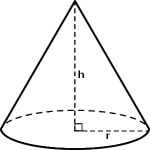
The radius of the disk becomes the slant height of the cone. The circumference of the disk is $2\pi \left( 1 \right)$ and so the circumference of the base of the cone is $C=2\pi \left( 1 \right)-x$ and its radius is $\displaystyle r=\frac{2\pi -x}{2\pi }=1-\frac{x}{2\pi }$ . The height, h of the cone is $\displaystyle h=\sqrt{1-{{\left( \frac{x}{2\pi } \right)}^{2}}}$ . See figure 4.

: Figure 3

: Figure 4

The volume of the cone is . $\displaystyle V=\frac{\pi }{3}{{\left( 1-\frac{x}{2\pi } \right)}^{2}}\sqrt{{{1}^{2}}-{{\left( 1-\frac{x}{2\pi } \right)}^{2}}}$

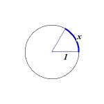
The graph of this equation is shown in Figure 5, and has two maximum values and a minimum. The domain appears to be $0<x<4\pi$ . But if $x>2\pi$ the piece you cut out will be larger than the original disk (and the expression under the radical will be negative). So our domain will be $0<x<2\pi$ (the endpoints correspond to not cutting any sector or cutting away the entire disk. The graph is shown in Figure 6 with, alas, only one extreme value.

: Figure 5

: Figure 6

(For the original expression the minimums are at $x=0,\ 2\pi ,\text{ and }4\pi$ and the maximums are at $x\approx 1.153\text{ and }x\approx 11.413$ . A CAS will help with these calculations or just use a graphing calculator.)

Extension 1: Find the value of x that will make the largest volume when the piece cut out is formed into a cone. Compare the two graphs and explain their congruence. See Figure 7.
Extension 2: Here I finally found what I was after. – a situation with more than one extreme value. Find the value of x that will make the largest total volume formed when the volume of the original cone and the cone formed by the piece cut out. Compare the first two graphs and the graph of this volume. See figure 8 – the magenta graph.

: Figure 7

: Figure 8

The Mae West Curve

There is at least one real situation that is modeled by a function with several extreme values. Spud’s blog gives the following explanation and illustration.

“When a Uranium (or Plutonium) atom fission, or splits, you end up with two much lighter atoms, called fission products, or daughter nuclides. The U-235 nucleus can split into a myriad of combinations, but some combinations are more likely than others.

“[Figure 9 below] shows the percentage of fission products by [atomic] mass[, A]. [This is] called the Mae West curve. … Note that the more likely fission products have two peaks at a mass of about 95 and 135.”

Thus we have a real life illustration of a model that has three extreme values in its domain.

The model graphed in Figure 9 is known as the “Mae West Curve,” named after Mae West (1893 – 1980) and actress, playwright and screenwriter.

: Figure 9: The “Mae West” Curve

If you know of any other real situations with more than one extreme, please let us know. Use the “comment” button below.

Continuous Fun

Posted on October 13, 2015 by Lin McMullin

The topic of this post is continuity. The phrase “a function is continuous on its domain” was much discussed last week on the AP Calculus Community bulletin board as it is about this time every year. This led to a discussion of one-sided continuity at the endpoint of an interval.

Let’s start by looking at some definitions related to continuity. A detailed discussion of definitions is worth doing in any math class; it helps students learn about the structure of mathematics. Definitions are biconditional statements; that is, either part implies the other.

Definitions related to Continuity

A function is continuous at a point, (a, f(a)) if, and only if, (1) f(a) exists (is a finite number), and (2) $\displaystyle \underset{x\to a}{\mathop{\lim }}\,f\left( x \right)$ exists (is a finite number), and (3) $\displaystyle \underset{x\to a}{\mathop{\lim }}\,f\left( x \right)=f\left( a \right)$ – the limit equals the value.

This is the three-part definition you will find in most textbooks. The first two conditions are sort of for emphasis since the third is not possible if the limit does not exist (or is infinite) and/or the value does not exist (DNE). Graphically this means that as you move along the graph of f getting closer to the place where x = a the function values are getting closer to f(a). This is not always the case; specifically, if this does not happen the function is not continuous at the point.

For example, let $\displaystyle f\left( x \right)=\frac{x-3}{(x-2)(x-3)}$

This function is undefined at x = 2 and x = 3; at both values f(x) DNE.
At x = 3 the limit does exist and is equal to 1. In this case the graph appears to be missing a single point, here (3, 1). This is called a removable discontinuity because be redefining the function so that f(3) = 1 the function could be made continuous. This happens most often when the factor in the denominator that becomes zero “cancels” with a like factor in the numerator. This can also happen if the function value is defined as something different than the limit. There are other examples such as $\displaystyle \frac{\sin \left( x \right)}{x}$ at x = 0
At x = 2 the limit DNE, and the situation appears as a vertical asymptote on the graph: on the left the values approach negative infinity and on the right they approach positive infinity. This is because a factor in the denominator gets very small as you approach 2.

Proving a function is continuous has been asked on AP Calculus exams. (See 2003 AB 6a and 2011 AB 6a) Students were expected to state the value of the two one-sided limits and the value of the function to show the three parts of the definition were true.

A function is continuous on an open interval if, and only if, it is continuous at every point in the interval.

The definition of continuous at a point is extended to all the points of an interval. But do you have to check each and every point? No, this is determined by finding where the function is not continuous; the function is then continuous on the intervals between these points.

In many theorems it is necessary to have a function be continuous on a closed interval; the endpoints must be included, but the limit in the main definition is a two-sided limit. The main definition is adapted to read A function is continuous from the right at x = a (or from the left at x = b) if, and only if, $\displaystyle \underset{x\to a+}{\mathop{\lim }}\,f\left( x \right)=f\left( a \right)\text{ }\left( \underset{x\to b-}{\mathop{\lim }}\,f\left( x \right)=f\left( b \right) \right)$ .

The limits are approached from inside the interval: from the right at the left end and from the left at the right end.

Continuous on its Domain

Functions exist only on their domain, so there is no way a function can be continuous except on its domain. I wrote about this is a previous post Right answer, Wrong Question.

When analyzing a new function one of the things you look for is where the function is continuous. But really you do this by looking for places where it is not continuous; everywhere else the function will be continuous.

Vertical asymptotes, removable discontinuities, and oscillating discontinuities are not possible for a function continuous on its domain; these appear on the graph, but mark places where the function DNE. The only kind of discontinuity a function may have on its domain are jump or step discontinuities. These often occur with piecewise defined functions where the endpoint of one piece is defined and different from the corresponding endpoint of the next piece. For example,

$\displaystyle f\left( x \right)=\left\{ \begin{matrix} \sin \left( x \right) & 0\le x\le \pi \\ \cos \left( x \right) & \pi <x\le 2\pi \\ \end{matrix} \right.$

Since $f\left( \pi \right)=0$ the function is defined there, but the limits of the two parts (0 and -1) are not the same, so the function is defined, but not continuous on its domain.

Another example is the greatest integer function (aka the floor function) whose graph is shown in below. Note that the left-endpoint of each segment (at the integer values) is included, while the right-endpoint at the next integer is not included.

Spotting discontinuities

Here are some hints on looking for places where a function is not continuous:

Look for the zeros of the denominators
For piecewise functions check the places where the pieces change definition.
For trigonometric functions, the sine and cosine are continuous for all x. Since the other trigonometric functions are defined in terms of the sine and cosine look places where the sine or cosine is zero and appears in the denominator of the definition.
Function involving square roots and other even degree roots are not defined, and therefore not continuous where their arguments are negative. For example, $\sqrt{4-{{x}^{2}}}$ is continuous on the closed interval [-2, 2] (using the definitions for closed intervals – one-sided limits), but not elsewhere.
Use technology to graph the function; discontinuities usually show up. The exception is a removable discontinuity or an oscillating discontinuity which may not show up because the x-value of the discontinuity may not be a pixel coordinate.

Pathological Examples

This function, attributed to Dirichlet, is defined for all Real numbers, but not continuous anywhere.

$f\left( x \right)=\left\{ \begin{matrix} 1 & \text{if }x\text{ is irrational} \\ 0 & \text{if }x\text{ is rational} \\ \end{matrix} \right.$

Between every pair of irrational numbers is a rational number, and between every pair of rational numbers is an irrational number.

With a slight variation, we have this function:

$\displaystyle g\left( x \right)=\left\{ \begin{matrix} 1 & \text{if }x\text{ is irrational} \\ x & \text{if }x\text{ is rational} \\ \end{matrix} \right.$

This function is defined for all Real numbers and is continuous at only one point (1, 1). Go figure.

Good Question 7 – 2009 AB 3

Posted on October 5, 2015 by Lin McMullin

Another in my occasional series on Good Questions to teach from. This is the Mighty Cable Company question from the 2009 AB Calculus exam, number 3

This question presented students with a different situation than had been seen before. It is a pretty standard “in-out” question, except that what was going in and out was money. Students were told that the Mighty Cable Company sold its cable for $120 per meter. They were also told that the cost of the cable varied with its distance from the starting end of the cable. Specifically, the cost of producing a portion of the cable x meters from the end is $6\sqrt{x}$ dollars per meter. Profit was defined as the difference between the money the company received for selling the cable minus the cost of producing the cable.

Students had a great deal of trouble answering this question. (The mean was 1.92 out of a possible 9 points. Fully, 36.9% of students earned no point; only 0.02% earned all 9 points.) This was probably because they had difficulty in interpreting the question and translating it into the proper mathematical terms and symbols. Since economic problems are not often seen on AP Calculus exams, students needed to be able to use the clues in the stem:

The $120 per meter is a rate. This should be deduced from the units: dollars per meter.
The cost of producing the portion of cable x meters from one end cable is also a rate for the same reason. In economics this is called the marginal cost; the students did not need to know this term.
The profit is an amount that is a function of x, the length of the cable.

Part (a): Students were required to find the profit from the sale of a 25-meter cable. This is an amount. As always, when asked for an amount, integrate a rate. In this case integrate the difference between the rate at which the cable sells and the cost of producing it.

$\displaystyle P(25)=\int_{0}^{25}{\left( 120-6\sqrt{x} \right)dx}=\$2500$

$\displaystyle P(25)=120(25)-\int_{0}^{25}{6\sqrt{x}\ dx}=\$2500$

Part (b): Students were asked to explain the meaning of $\displaystyle \int_{25}^{30}{6\sqrt{x}dx}$ in the context of the problem. Since the answer is probably not immediately obvious, here is the reasoning involved.

This is the integral of a rate and therefore, gives the amount (of money) needed to manufacture the cable. This can be found by a unit analysis of the integrand: $\displaystyle \frac{\text{dollars}}{\text{meter}}\cdot \text{meters}=\text{dollars}$ .

Let C be the cost of production, so $\displaystyle \frac{dC}{dx}=6\sqrt{x}$ , and therefore, $\displaystyle \int_{25}^{30}{6\sqrt{x}dx}=C\left( 30 \right)-C\left( 25 \right)$ by the Fundamental Theorem of Calculus (FTC).

Therefore, $\displaystyle \int_{25}^{30}{6\sqrt{x}dx}$ is the difference in dollars between the cost of producing a cable 30 meters long, C(30), and the cost of producing a cable 25 meters long, C(25). (Another acceptable is that the integral is the cost in dollars of producing the last 5 meters of a 30 meter cable.)

Part (c): Students were asked to write an expression involving an integral that represents the profit on the sale of a cable k meters long.

Part (a) serves as a hint for this part of the question. Here the students should write the same expression as they wrote in (a) with the 25 replaced by k.

$\displaystyle P(k)=\int_{0}^{k}{\left( 120-6\sqrt{x} \right)dx}$

$\displaystyle P(k)=120k-\int_{0}^{k}{6\sqrt{x}\ dx}$

Part d: Students were required to find the maximum profit that can be earned by the sale of one cable and to justify their answer. Here they need to find when the rate of change of the profit (the marginal profit) changes from positive to negative.

Using the FTC to differentiate either of the answers in part (c) or by starting fresh from the given information:

$\displaystyle \frac{dP}{dx}=120-6\sqrt{x}$

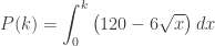
$\displaystyle \frac{dP}{dx}=0$ when x = 400 and P(400)= $16,000.

Justification: The maximum profit on the sale of one cable is $16,000 for a cable 400 meters long. For $0<x<400,{P} '(x)>0$ and for $x>400,{P} '(x)<0$ therefore, the maximum profit occurs at x = 400. (The First Derivative Test).

Once students are familiar with in-out questions, this is a good question to challenge them with. The actual calculus is not that difficult or unusual but concentrating on the translation of the unfamiliar context into symbols and calculus ideas is different. Show them how to read the hints in the problem such as the units.

Steel cable or steel wire rope as it is called also has some interesting geometry in its construction. You can find many good illustrations of this, such as the ones below, by Googling “steel wire rope.”

This slideshow requires JavaScript.

October 2015

Posted on October 1, 2015 by Lin McMullin

A personal note: My wife and I just moved from Texas back to Saratoga County, New York where I spend 29 years teaching. My seven and one-half years in Texas were a lot of fun. I had the opportunity to travel all over the USA from Boston to Honolulu, working with calculus teachers, which I really enjoyed. But we just missed the snow and taxes, so here we are. We spent the last six weeks or so traveling the country. That was not quite our plan, but our new house was still under construction and not ready. Today, we moved in; in a few days our furniture will arrive from Texas – we hope.

I guess this will make me re-semi-retired (if that’s a word). I’ll still be writing and doing workshops and whatever else comes along.

He is the list of topic that may be of interest in October. Most were written in the first year (2012) when I was trying to go through the curriculum more-or-less in order staying a little ahead of where I figured you would be. So they should be useful now. Others were written later and are included since they fit in the order. The four on the main page under this one are the most popular from October in the last year. “Reading the Derivative’s Graph” remains the all-time high with over 3200 hits.

October 1, 2012, The Mean Value Theorem II

August 18, 2014 Darboux’s Theorem

October 3, 2012 Derivative Practice – Numbers

October 5, 2012 Derivative Practice – Graphs

October 8, 2012 Related Rate Problems I

October 10, 2012 Related Rate Problems II

October 12, 2012 Why Radians?

October 15, 2012 Concepts Related to Graphs

October 17, 2012 The Shapes of a Graph

October 19, 2012 Joining the Pieces of a Graph

October 22, 2012 Extreme Values

October 23, 2104 The Marble and the Vase An extreme value problem.