
Don’t get me wrong; finding volumes of solids of rotation by the method of cylindrical shells is a great method. It’s just that you can always work around it; you don’t ever need to use it. The work-around is often longer and involves more work, but it is interesting mathematically. So here’s an example of how to do it.
The region bounded by the graph of 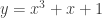
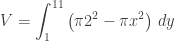
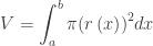
Supposedly this volume must be found by the shell method. Using the washer method the volume is set up as the integral of the area of the outside circle with constant radius of 2, minus the area of the inside circle of radius x, times the “thickness” of a slice. This “thickness” is in the y-direction and so is dy. The dy also determines the limits of integration.
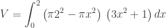
Since the integral contains a dy the usual way is to change the x to a function of y, which in this case involves solving a cubic polynomial. In this case that is very difficult to find x as a function of y and with a different function that may even be impossible. But do we really have to do that? In fact, what is required is to have only one variable and the variable may be x! So we find dy in terms of x and dx and substitute into the expression above. We also change the limits of integration to the corresponding x-values.

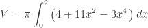
This integral is easy to evaluate and will give the same value, 
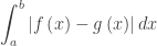
To use this idea, the function must either be one-to-one on the interval or the solid must be broken into sections that are one-to-one. This may make the problem longer. Most problems that you want to do by shells are easier by shells. The point is that washers (or disks) may always be used; not that the washer approach is the easiest way.
 from x = 0 to
 ; the thickness is
 .
. ) from the outside volume (radius =
  ). This may be done with two integrals or combined into one.
 is often factored out in front of the integral sign to make things look neater; I suggest you leave it where it is to remind students that they are subtracting the areas of two circles.
 .
. .
. .
.

 .
.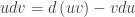 .
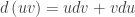
.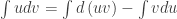 . By the FTC the first term on the right can be simplified giving the formula for Integration by Parts:
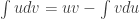
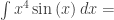
 in which there is a combination of functions that are usually of different types – here a polynomial and a trig function.
 . Here we make the substitutions
 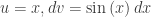 and from these we compute
  . (There is no need for the +C here; it will be included later). Making these substitutions gives

 and
and  the result is
