
Using Local Linearity to introduce difference quotient and the derivative.
An effective way to introduce difference quotients and derivatives is to write the equation of the “line” you see when you zoom-in on a locally linear function.
First: Ask your class to use their calculator or computer grapher to graph a function, say y = sin(x), or some function they like better.
- Ask them to trace over to some point where the graph is “curvy.” (So they will remain on the graph, use the TRACE feature, not the moving cursor.) They do not have to go to, or even be near, the same place.
- Then ask them to zoom-in several times until their graph looks like a straight line (locally linear) and save the coordinates of that point as a and b (see the technology hint below).
- Then return to the graph and trace one or two clicks left or right to a nearby point on the graph and record the coordinates of that point as c and d.
- Write the equation of the line through (a, b) and (c ,d) and enter it in the graphing menu (see technology hint again).
- Graph the line. They should see only one “line” because the two graphs are on top of each other.
- Re-graph in the standard or Trig window. What do you see now? They should see their original graph with a line that appears tangent to it at the point (a, b).
Next: Discuss what you’ve done, specifically in finding the slope. The value c is a plus a little bit, that is c = a + h. (Or minus a little bit if h is negative.) So the slope is
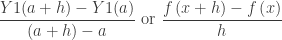
and now you are ready to talk about difference quotients and their limit the derivative.
Technology Hints:
When you trace a graph on a calculator the coordinates of the point are written on the bottom of the screen as X and Y, or xc and yc. If you return to the home screen and type X [STO] A and Y [STO] B (or xc [STO] a etc.) the values will be saved to A and B. When you trace to the next point the x and y change, so return to the home screen and save them as C and D.
The line can be written directly in the equation editor in point-slope form by typing Y2 = Y1(A) + (Y1(B)-Y1(A))/(B – A)*(x – A)
 and
and  . Maybe that will lessen the confusion there.
