The parametric/vector equation questions only concern motion in a plane.
In the plane, the position of a moving object as a function of time, t, can be specified by a pair of parametric equations 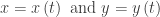

The velocity of the movement in the x- and y-direction is given by the vector 
The length of this vector is the speed of the moving object. 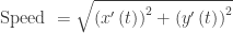

The acceleration is given by the vector 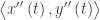
What students should know how to do:
- Vectors may be written using parentheses, ( ), or pointed brackets,
, or even
form. The pointed brackets seem to be the most popular right now, but all common notations are allowed and will be recognized by readers.
- Find the speed at time t:
- Use the definite integral for arc length to find the distance traveled
. Notice that this is the integral of the speed (rate times time = distance).
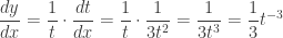
- The slope of the path is
. See this post for more on finding the first and second derivatives with respect to x.
- Determine when the particle is moving left or right,
- Determine when the particle is moving up or down,
- Find the extreme position (farthest left, right, up, down, or distance from the origin).
- Given the position find the velocity by differentiating; given the velocity find the acceleration by differentiating.
- Given the acceleration and the velocity at some point find the velocity by integrating; given the velocity and the position at some point find the position by integrating. These are just initial value differential equation problems (IVP).
- Dot product and cross product are not tested on the BC exam, nor are other aspects.
When this topic appears on the free-response section of the exam there is no polar equation question and vice versa. When not on the free-response section there are one or more multiple-choice questions on parametric equations.
Free-response questions:
- 2012 BC 2
- 2016 BC 2
Multiple-choice questions from non-secure exams
- 2003 BC 4, 7, 17, 84
- 2008 BC 1, 5, 28
- 2012 BC 2
 from the first. (From the previous posts: if
  then there are d dips, loops, or cusps in n full revolutions). Both graphs will have the same R value.


 , R = 0.00667 and slightly less than a full revolution. Make the image size (under the file tab) 12.3 x 12.3 (the units are cm.), or 465 x 465 pixels (type @ after the number to use pixels). Amazing!
 and,
and,  then the tradition formula gives
 , and
, and
 , that bothers me. Where did the
 is a function of t you must begin by differentiating the first derivative with respect to t. Then treating this as a typical Chain Rule situation and multiplying by
  exists.)
 and
and 
 , and
, and  and
and  .
.