Graphing Taylor Polynomials

The eighth in the Graphing Calculator / Technology series

Here are some hints for graphing Taylor polynomials using technology. (The illustrations are made using a TI-8x calculator. The ideas are the same on other graphing calculators; the syntax may be slightly different.)

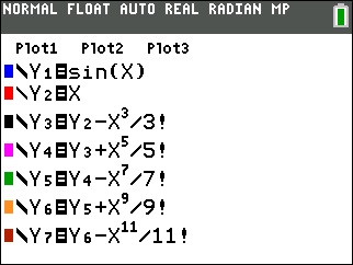
Each successive term of a Taylor polynomial consists of all the previous terms plus one new term. To show students how Taylor polynomials closely approximate a function (in the interval of convergence, of course), enter the function as Y1. Then enter the first term of the polynomial as Y2. Enter the next polynomial as Y3 = Y2 + the second term; enter the next as y4 = Y3 + the next term, and so on.

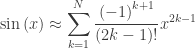
The example is the McLaurin series for sin(x) centered at the origin:

\displaystyle \sin \left( x \right)=x-\frac{{{x}^{3}}}{3!}+\frac{{{x}^{5}}}{5!}+\cdots +\frac{{{(-1)}^{2n-1}}{{x}^{2n-1}}}{\left( 2n-1 \right)!}=\sum\limits_{n=1}^{\infty }{{{\left( -1 \right)}^{n+1}}\frac{{{x}^{2n-1}}}{\left( 2n-1 \right)!}}

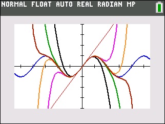
Each will graph one at a time. Watching them graph, one at a time, is instructive as well; each curve approximates the sine curve (in black) further and further away from the origin.

series-1

series-2

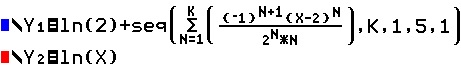
Another way to graph the polynomials is to enter them as a sequence of sums. The example this time is ln(x) centered at x = 2:

\displaystyle \ln \left( x \right)=\ln \left( 2 \right)+\frac{x-2}{2}-\frac{{{\left( x-2 \right)}^{2}}}{8}+\frac{{{\left( x-2 \right)}^{3}}}{24}+...=\ln \left( 2 \right)+\sum\limits_{n=1}^{\infty }{{{\left( -1 \right)}^{n+1}}\frac{{{\left( x-2 \right)}^{n}}}{{{2}^{n}}n}}

The syntax is seq( series in sigma notation, indexing variable, start value, end value [,step]). Notice from the figure that the indexing variable, K, is above the sigma.

series-4

The individual polynomials graph in the same color (blue); the function is shown in red.

series-3
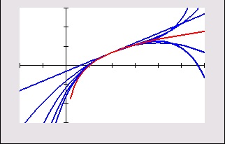
Comparing the two graphs (sin(x) and ln(x)) is a good way to start a discussion about the interval of convergence – ask what is different about the graphs as more polynomials are graphed on each. Notice that unlike the sin(x) series the ln(x) polynomials only come close to the function in a limited interval (0, 4) centered at x = 2.


Desmos is also a good program to use to illustrate Taylor and McLaurin polynomials (as are Geogebra and Winplot). The use of the sliders makes it possible to see the successive polynomials quickly. They also help students see the interval of convergence as higher degree polynomials hug the graph on wider intervals (sin(x)), or stay within the same interval (ln(x)). The Desmos illustration with slider for the sin(x) centered at the origin is here and for ln(x)  centered at x = 2 is here. Study the input on the left side and enter Taylor polynomials for other functions.

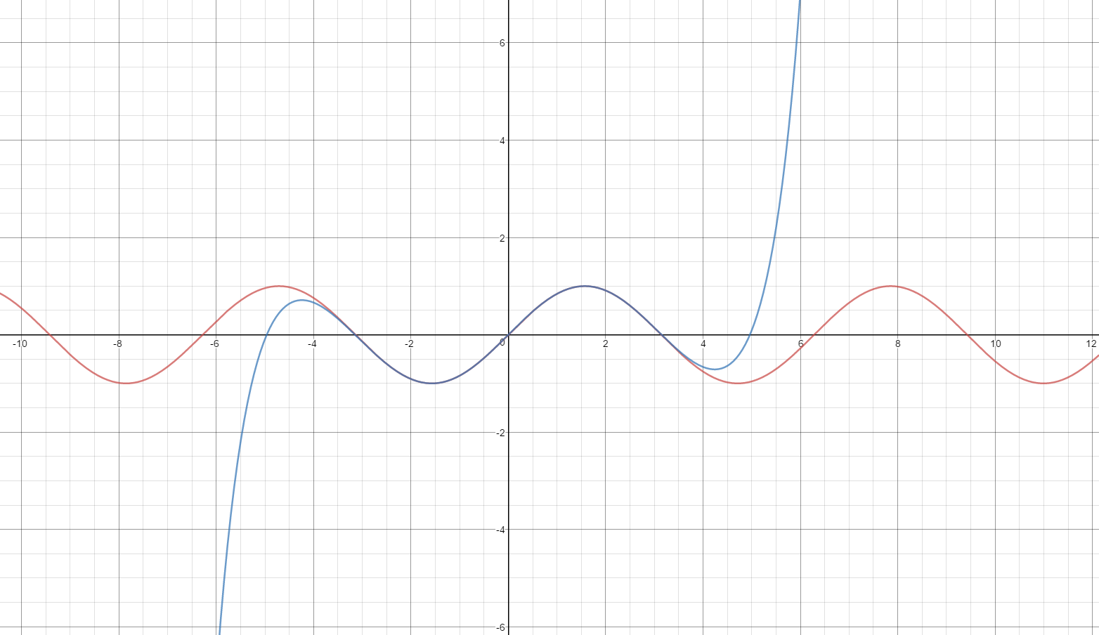
The fifth degree Taylor polynomial for sin(x) centered at the origin.The interval of convergence is all real numbers. Each polynomial “hugs” the graph on wider intervals.

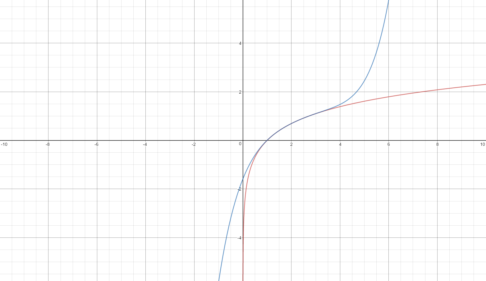
The fifth degree Taylor polynomial for ln(x) centered at x = 2. The interval of convergence is 0 < x < 4. The polynomials all leave the graph outside of this interval.


Coming soon

Feb 14th, Geometric Series – Far Out


Advertisement

Everyday Series

A Square Root

A Square Root

Our BC friends will soon be starting to teach series. Today, to emphasize that series are all around us, I would like to discuss series that we see every day: numbers.

Long ago I was taught that no one has ever seen a “number.” Have you ever seen a four? What we see are numerals, symbols or words that represent a number. These symbols come in two types: decimals and others. The others are better described as directions for finding the decimal representation. For example, ½ tells you to divide 1 by 2, that will give the decimal 0.5.

The place-value (decimal) representation of a number is a shortcut (and a nice one) for a series that gives the value of the number. Here 4203.876 is written as a finite series, or, if you prefer, an infinite series with the remaining terms all zero.

4203.876=4\left( {{10}^{3}} \right)+2\left( {{10}^{2}} \right)+0\left( {{10}^{1}} \right)+3\left( {{10}^{0}} \right)+8\left( {{10}^{-1}} \right)+7\left( {{10}^{-2}} \right)+6\left( {{10}^{-3}} \right)

Repeating decimals can also be written as infinite series. The first step is to follow the “directions” and divide 23 by 99:

\displaystyle \frac{23}{99}=0.23\overline{23}=\sum\limits_{n=1}^{\infty }{\left( 2\left( {{10}^{1-2n}} \right)+3\left( {{10}^{-2n}} \right) \right)}

Irrational numbers are a little different. What are they anyway? Where do they go on the number line? The decimal approximations will tell us that.

I will demonstrate a way of finding the decimals with a simple example \sqrt{2}. (There are many algorithms for doing this (see especially the digit-by-digit calculation), but it only applies to square roots and doesn’t really tell us what \sqrt{2} means.) The approach below lets us see what is going on.

The square root of two is the number that when multiplied by itself equals 2. The sequence 1, 1.4, 1.41, 1.414, 1.4142, 1.41421, 1.414213. … gives successively better approximation to \sqrt{2}.

Each successive number is found this way. At any place in the sequence the next number must one decimal place longer and end with one of the digits 0, 1, 2, 3, …, or 9.

Let’s try 6: 1.41421362 = 2.00000010642496 Too big!

So, let’s try 5: 1.41421352 = 1.99999982358225 Too small.

We’ll use the smaller one and then compute the next digit the same way: try digits until we find the largest digit that gives a square less than 2. (Or we could use the smallest digit that gives a result largest than 2; I’ll discuss that below.)

If we continue this way we will end up with a non-decreasing sequence, since putting a digit on the end always gives a slightly larger number, except for the digit zero which gives the same number. This series is also bounded (all the values are greater than 1 and less than 2).  Such a series must converge to its least upper bound. For this series, the least upper bound is the number we call \sqrt{2}; the number defined as \sqrt{2}.

Consider the series 2, 1.5, 1.42, 1,415, 1,4143, 1,41422, 1,414214, … in which each term has for its last digit one more than the corresponding term in the previous series above. This series is non-increasing and bounded, and, therefore, converges to its greatest lower bound, the same number \sqrt{2}.

In a way, these series define \sqrt{2}.

This is not a very efficient way to find values. Some irrational numbers, like π or e, cannot be found this way. But that is not the point. The point is that all numbers have a decimal representation. This decimal representation is a shorthand way of writing the finite or infinite series that converges to the number. Since we cannot write all the decimals for many numbers, the decimal form gives a series of gives better and better approximations.

So sequences and series are all around us every day.


A more formal approach goes like this. Let {{S}_{k}} 
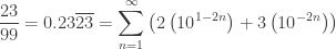
be the k-place decimal found as described above for the first series. Then {{S}_{k}}+{{10}^{-k}} will be the k­-place decimal whose last digit is one more than the last digit of {{S}_{k}} . Then {{S}_{k}}^{2}<2<{{\left( {{S}_{k}}+{{10}^{-k}} \right)}^{2}} and {{S}_{k}}<\sqrt{2}<{{S}_{k}}+{{10}^{-k}},. This implies 0<\sqrt{2}-{{S}_{k}}<{{10}^{-k}}. Since {{10}^{-k}} can be made as small as we want, \underset{k\to \infty }{\mathop{\lim }}\,\left( \sqrt{2}-{{S}_{k}} \right)=0 and \underset{k\to \infty }{\mathop{\lim }}\,{{S}_{k}}=\sqrt{2}. The series converges to \sqrt{2}.


How the mind works (or at least how my mind works when it’s working):

None of this is original to me. Maybe I learned it years ago in college or graduate school; if so, I had forgotten it long ago. Four or five years ago while I was living in Texas, I started reading Calculus Deconstructed – A Second Course in First-year Calculus by Zbigniew Nitecki. He discusses this approach in a much more formal way without the example. In thinking about writing on this topic recently, I outlined the example above in my head (which is what I do when I’m trying to fall asleep). You can see where I ended up. While nothing like Nitecki’s work, it is the same idea.

I find this strange and fascinating: I absorbed that and put it all together in a different way without thinking about it in the intervening years. Strange how the mind works.


Coming soon:

  • Jan 24th, Logistic Growth – Real and Simulated
  • Jan 31st, The Logistic Equation
  • Feb 7th, Graphing Taylor Polynomials
  • Feb 14th,  Geometric Series – Far Out

February 2016

As I hope you’ve noticed there is a new pull-down on the navigation bar called “Website.” For some years I’ve had a website at linmcmullin.net that lately I’ve been neglecting. I decided to close it in the next few days, and therefore, I move most of the material that is there to this new tab. The main items of interest are probably those under “Calculus”, “Winplot”, and “CAS.” If you used that website you should be able to find what you need here. If you cannot find something, then please write and I’ll try to help.

In my post entitled January 2016 are listing of post for the applications of integration for both AB and BC calculus. This month’s posts are BC topics on sequences, series, and parametric and polar equations.

Posts from past Februarys

Sequences and Series

February 9, 2015 Amortization A practical application of sequences.

February 8, 2013: Introducing Power Series 1

February 11, 2013: Introducing Power Series 2

February 13, 2013: Introducing Power Series 3

February 15, 2013 New Series from Old 1

February 18, 2013: New Series from Old 2

February 20, 2013: New Series from Old 3

February 22, 2013: Error Bounds

May 20, 2015 The Lagrange Highway

Polar, Parametric, and Vector Equations

March 15, 2013 Parametric and Vector Equations

March 18, 2013 Polar Curves

May 17, 2014 Implicit Differentiation of Parametric Equations 

A series on ROULETTES some special parametric curves (BC topic – enrichment):


Introducing Power Series 1

The next few posts will discuss a way to introduce Taylor and Maclaurin series to students. We will kind of sneak up on the idea without mentioning where we are going or using any special terms. In this post we will find a way of approximating a function with a polynomial of any degree we choose. In the next post we will look at the graph of these polynomials and finally suggest some questions for further thought.

Making Better Approximations

Students already know and have been working with the tangent line approximation of a function at a point (a, f(a)):

f(x)\approx f\left( a \right)+{f}'\left( a \right)\left( x-a \right)

ln(x):

For the function f\left( x \right)=\ln \left( x \right) at the point (1, 0) ask your students to write the tangent line approximation: y=0+(1)(x-1) .Point out that this line has the same value as  ln(xand its derivative as at (1, 0).

Then suggest that maybe having a polynomial that has the same value, first derivative and second derivative might be a better approximation. Suggest they start with y=a+b\left( x-1 \right)+c{{\left( x-1 \right)}^{2}} and see if they can find values of a, b and c that will make this happen.

Since f\left( 1 \right)=0,{f}'\left( 1 \right)=1\text{ and }{{f}'}'\left( x \right)=-1 we can write

y=a+b\left( x-1 \right)+c{{\left( x-1 \right)}^{2}};\quad y\left( 1 \right)=a+0+0=0;\quad a=0

{y}'=b+2c\left( x-1 \right);\quad {y}'\left( 1 \right)=b+0=\tfrac{1}{1};\quad b=1

{{y}'}'=2c;\quad {{y}'}'\left( 1 \right)=c=-\tfrac{1}{{{1}^{2}}}=-1;\quad c=-\tfrac{1}{2}

y=0+\left( x-1 \right)-\tfrac{1}{2}{{\left( x-1 \right)}^{2}}

Then suggest they try a third degree polynomial starting with y=a+b\left( x-1 \right)+c{{\left( x-1 \right)}^{2}}+d{{\left( x-1 \right)}^{3}}. Proceeding as above, all the numbers come out the same and we find that

\ln \left( x \right)\approx 0+\left( x-1 \right)+\left( -\tfrac{1}{2} \right){{\left( x-1 \right)}^{2}}+\left( \tfrac{1}{3} \right){{\left( x-1 \right)}^{3}}

Then go for a fourth- and fifth-degree polynomial until they discover the patterns. (The signs alternate, and the denominators are the factorial of the exponent.)

See if the class can write a general polynomial of degree N :

 \displaystyle \ln \left( x \right)\approx \sum\limits_{k=1}^{N}{\frac{{{\left( -1 \right)}^{k+1}}}{k}{{\left( x-1 \right)}^{k}}}

sin(x):

Then have the class repeat all this for a new function such as f\left( x \right)=\sin \left( x \right) at the point (0, 0). This could be assigned as homework or group work. Ask them to do enough terms until they see the pattern. There will be patterns similar to ln(x ) and every other term (the even powers) will have a coefficient of zero.

\sin \left( x \right)\approx x-\tfrac{1}{3!}{{x}^{3}}+\tfrac{1}{5!}{{x}^{5}}-\tfrac{1}{7!}{{x}^{7}}+\tfrac{1}{9!}{{x}^{9}}

or in general the polynomial of degree N is

\displaystyle \sin \left( x \right)\approx \sum\limits_{k=1}^{N}{\frac{{{\left( -1 \right)}^{k+1}}}{\left( 2k-1 \right)!}{{x}^{2k-1}}}

How good is this approximation? Using only the first three terms of the polynomial above you will tell you that. Pretty close: correct to 5 decimal places.  Using four terms gives correct to 7 decimal places when rounded.

Finally, see if they can generalize this idea to any function f at any point on the function \left( {{x}_{0}},f\left( {{x}_{0}} \right) \right). This time you will not have the various derivatives as numbers, rather they will be expressions like . Work through the powers one at a time to go from y=a+b\left( x-{{x}_{0}} \right)+c{{\left( x-{{x}_{0}} \right)}^{2}}+d{{\left( x-{{x}_{0}} \right)}^{3}}+e{{\left( x-{{x}_{0}} \right)}^{4}}

and so on, until you get to

f\left( x \right)\approx f\left( {{x}_{0}} \right)+\frac{{f}'\left( {{x}_{0}} \right)}{1!}\left( x-{{x}_{0}} \right)+\frac{{{f}'}'\left( {{x}_{0}} \right)}{2!}{{\left( x-{{x}_{0}} \right)}^{2}}

\quad \quad \quad \quad \quad \quad \quad \quad \quad \quad \quad \quad \quad +\cdots +\frac{{{f}^{\left( N \right)}}\left( {{x}_{0}} \right)}{N!}{{\left( x-{{x}_{0}} \right)}^{N}}

For example the third derivative computation would look like this:

{{{y}'}'}'=3\cdot 2\cdot 1d+4\cdot 3\cdot 2e\left( x-{{x}_{0}} \right)

{{{y}'}'}'\left( {{x}_{0}} \right)=3\cdot 2\cdot 1d+4\cdot 3\cdot 2e(0)={{{f}'}'}'\left( {{x}_{0}} \right)

d=\frac{{{{f}'}'}'\left( {{x}_{0}} \right)}{3!}

The computations here are perhaps a little different than what students have seen, so take your time doing this. Two or even three class days may be necessary.

Notice these things:

  • The first two terms are the tangent line approximation.
  • The various derivatives are numbers that must be calculated.
  • All the terms of any degree are the same as the terms of the previous degree with one additional term.

Next post in this series: Looking at all this graphically.

(Typos in an earlier version of this post have been corrected – LMc)