Difference Quotients

Difference quotients are the path to the definition of the derivative. Here are three posts exploring difference quotients.

Difference Quotients I  The forward and backward difference quotients

Difference Quotients II      The symmetric difference quotient and seeing the three difference quotients in action.  Showing that the three difference quotients converge to the same value.

Seeing Difference Quotients      Expands on the post immediately above and shows some numerical and graphical approaches using calculators and Desmos.

 Tangents and Slopes You can use this Desmos app now to preview some of the things that he tangent line can tell us about the graph of a function or save (or reuse) it for later when concentrating on graphs. Discuss slope in relation to increasing, decreasing, concavity, etc.

At Just the Right Time

Stamp out Slope-intercept Form


Working up to the derivative.

While limit is what makes all of the calculus work, people usually think of calculus as starting with the derivative. The first problem in calculus is finding the slope of a line tangent to a graph at a point and then writing the equation of that tangent line.

Local Linearity is the graphical manifestation of differentiability. If you zoom-in of the graph of a function (at a point where we will soon say the function is differentiable), the graph eventually looks like a line: the graph appears to be straight, and its slope is the number we will call its derivative.

To do this we need to zoom-in numerically. Zooming-in numerically is accomplished by finding the slope of a secant line, a line that intersects the graph twice, and then finding the limit of that slope as the two points come closer together.

This week’s posts start with local linearity and tangent lines. They lead to the difference quotient and the equation of the tangent line.

Local Linearity I

Local Linearity II      Working up to difference quotient. The next post explains this in more detail.

Tangent Lines approaching difference quotients on calculator by graphing tan line.

Next week: Difference Quotients.


Seeing Difference Quotients

Third in the graphing calculator series. 

In working up to the definition of the derivative you probably mention difference quotients. They are

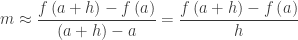
The forward difference quotient (FDQ): \displaystyle \frac{f\left( x+h \right)-f\left( x \right)}{h}

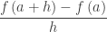
The backwards difference quotient (BDQ): \displaystyle \frac{f\left( x \right)-f\left( x-h \right)}{h}, and

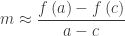
The symmetric difference quotient (SDQ): \displaystyle \frac{f\left( x+h \right)-f\left( x-h \right)}{2h}

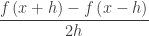
Each of these is the slope of a (different) secant line and the limit of each as, if it exists, is the same and is the derivative of the function f at the point (x, f(x)). (We will assume h > 0 although this is not really necessary; if h < 0 the FDQ becomes the BDQ and vice versa.)

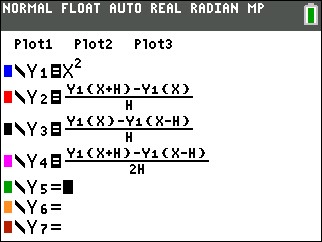
To see how this works you can graph a function and the three difference quotients on a graphing calculator. Here is how. Enter the function as the first function on your calculator and the difference quotients with it. Each of the difference quotients is defined in terms of Y1; this allows us to investigate the difference quotients of different functions by changing only Y1.

DQ 1

Now, on the home screen assign a value to h by typing [1] [STO] [alpha] [h]

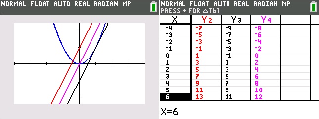
Graph the result in a square window.

The look at the table screen. (Y1 has been turned off). Can you express Y2, Y3, and Y4 in term of x?

DQ 2

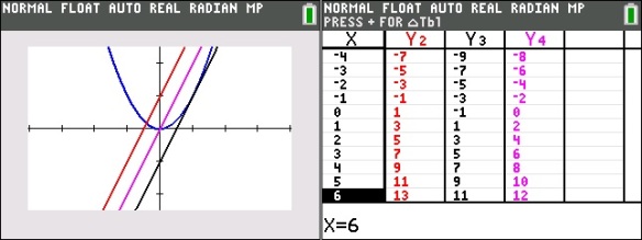
Then change h by storing a different value, say ½, to h and graph again. Then look at the table screen again. Can you express Y2, Y3, and Y4 in term of x?

DQ 3

Then graph again with h = -0.1

DQ 4

As you can see as h gets smaller (h 0), the three difference quotients are FDQ: 2x + h, the BDQ is 2x – h, and the SDQ is 2x. They converge to the same thing. The limit of each difference quotient as h approaches zero is twice the x coordinate of the point. If you’re not sure try a smaller value of h.

The function to which each of these converge is called the derivative of the original function (Y1). In the example the derivative of x2 is 2x.

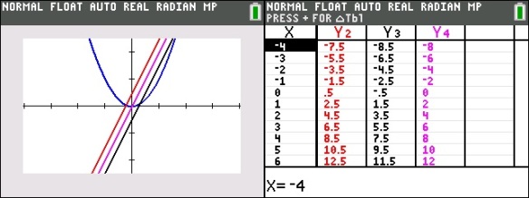
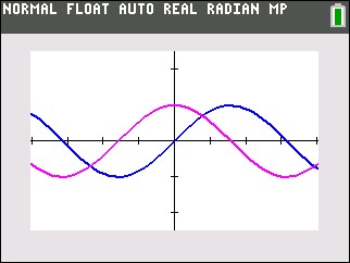
Now try another function say, Y1 = sin(x) and repeat the graphs and tables above. The tables will probably not be of much help, since the pattern is not familiar. The graph shows the function (dark blue) and only the SDQ (light blue), h = 0.1 Can you guess what the derivative might be?

DQ 5

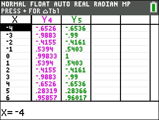
I f you guessed cos(x) you are correct. The table shows the SDQ values as Y4, and the values of cos(x) as Y5. Pretty close! If you want to get closer try h = 0.001.

DQ 6

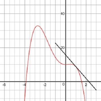
If you have a CAS calculators such as the TI-Nspire or the HP PRIME you can do this activity with sliders. Also you may try this with DESMOS. Click here or on the graph below. Some interesting functions to start with are cos(x) and | x |.

And by the way, the SDQ is what most graphing calculators use to calculate the derivative. It is called nDeriv on TI calculators.

Discovering the Derivative

Discovering the Derivative with a Graphing Calculator

This is an outline of how to introduce the idea that the slope of the line tangent to a graph can be found, or at least approximated, by finding the slope of a line through two very close points in the graph.  It is a set of graphing calculator activities that will use graphs and numbers to lead to the symbolic form of the derivative.

You may work through the activities with your class (which is what I would do) or you could write and distribute them and let your class do them a laboratory exercise. Before starting students should know how to use their calculator to graph, to trace to points on the graph, and how to save and recall the coordinates from the graph to variables on the home screen using the graphing calculator’s store feature.

I suggest you work through these three times (or more) using different functions. I will work with y={{x}^{2}}. A good second example is y={{x}^{3}}, and a third example to use is y=\sin \left( x \right). Use simple functions, because you will want the students to see the answers without too much trouble.The procedure is the same for all.

Part 1:

  1. Begin by asking students to entery={{x}^{2}} in their calculator asY1 and graph it in a standard, square window. (Do not use the decimal window as “nice” decimals are not necessary or helpful.)

    GC Derivative 1

    Figure 1

  2. Next, have them trace over to different points on the graph (some should go left and others to the right); they should all end up at different points. Then have them zoom-in 6 or 8 times until the graph looks linear. (This is local linearity – functions that are differentiable are locally linear.)
  3. Then push TRACE to be sure the cursor is on the graph. The coordinates of the point are on the bottom of the screen. Go to the HOME screen and save the two values as a and b. Think of this first point as (a, b).
  4. Return to the graph screen and push TRACE. This should return the cursor to the first point. (If not, close is okay.) Then click to the right or to left once, or twice at most, to move to a nearby point on the graph. Return to the home screen and save the new values to c and d for the second point (c, d).
  5. On the home screen use a, b, c, and d to write the slope of the line through the two points. See figure 1. (Go around the room as they are doing this and make sure students are getting this – their slope should be approximately twice a or c.)
  6. Return to the equation screen and enter the equation of the line through the two points asY2. (See figure 2). Graph this equation with the parabola.

    Figure 2

    Figure 2

  7. Have the students record their values of a, b, c, d and m on paper (three decimal places will be enough) and also write a description of what they see on the graph and why they think this is so. (This is in case they lose the numbers on their calculator when they do another graph and also because you will need them later in the next part of the exploration.)

Repeat the same steps separately with the other two functions and record the results in the same way. Write their numbers and observations. Discuss the observations with the class.

  • Of course, the lines should look tangent to the graphs, but since they contain two points of the graph, they cannot actually be tangent.
  • Discuss how a line can be tangent to a graph. How is this different from a tangent to a circle?
  • Ask what could be done to make their line even closer to being tangent. (Use points closer together.)

Part 2:

Now you have homework to do. Collect the student’s data and combine it into a list with columns for a, c, and m. The points do not have to be in order. Leave any “wrong” points for discussion; if there are none, you might want to make one up and include it. Do this for each of the three sets of data. Make a copy for each student. Enter the numbers for a and m as lists in your emulator and make a dot-plot of the points (a, m) = (a, slope at x = a).

  1. Return the lists of points to the students and ask them to study the list and see if they can see any obvious relationship between the numbers on each line. Answers for y = x2 should be the m is approximately twice either a or c; or maybe some will see that m is approximately a + c. Answers for y = x3 will be less obvious (three times the square of a). Answers for y = sin(x) will not be obvious at all.
  2. Using the emulator, separately for each of the three sets of data, make a dot-plot of the numbers (use a square window). Ask the student to discuss what they see. See if they can find an equation of the graph of the dot-plots. Now the equation of the data set for sin(x) should be obvious. Plot their guesses on top of the points and see how close they come.

Part 3:

Now guide the class through the symbolic explanation of what they did. Ask them to explain and write in symbols specifically what they did. The idea here is for you, the teacher, to ask lots of leading questions until the class decides on the best answer.

  1. Call the first point (a, f(a)). Let h = “a little bit.” then the second is the point (a plus a little bit, f(a plus a little bit)) or (a + h, f(a + h)). Recall that h may have been negative for some students so the second point may actually be to the left of the first. Then help them come up with

\displaystyle m\approx \frac{f\left( a+h \right)-f\left( a \right)}{\left( a+h \right)-a}=\frac{f\left( a+h \right)-f\left( a \right)}{h}

Or they may prefer

\displaystyle m\approx \frac{f\left( a \right)-f\left( c \right)}{a-c}

  1. Ask how this could be made “less approximate” and more actually equal. (Answer: smaller and smaller value of h.) Ask them to find the value of h = ac for their points. How small are they? How can you make them really small? (Find a limit.)
  2. Notice that h cannot be zero in these expressions. Keep hinting until someone comes up with the idea of finding

\displaystyle \underset{h\to 0}{\mathop{\lim }}\,\frac{f\left( a+h \right)-f\left( a \right)}{h}  or  \displaystyle \underset{a\to c}{\mathop{\lim }}\,\frac{f\left( a \right)-f\left( c \right)}{a-c}

  1. Next have the students calculate the limits below by actually doing the algebra. (They will not be able to handle the sin(x) at this point so save that for later.)

\displaystyle \underset{h\to 0}{\mathop{\lim }}\,\frac{{{\left( x+h \right)}^{2}}-{{\left( x \right)}^{2}}}{h}\text{ and }\underset{h\to 0}{\mathop{\lim }}\,\frac{{{\left( x+h \right)}^{3}}-{{\left( x \right)}^{3}}}{h}

  1. Compare the answers here with the earlier work and guesses, and discuss.

… And now you are ready to define the limits as the ’(a) derivative of f at x = a.

.

The Derivative II

(In this activity I am paraphrasing and expanding the suggestions of Alan Lipp in a posting “Derivatives of Trig Functions” August 29, 2012 to the Calculus Electronic Discussion Group.)

This activity parallels the one in my last post here using technology.

    1. Enter the function you are investigating as Y1 in your calculator. Later you will change this to other functions but will not have to change the following entries.  Start with Y1 = x2.
    2. Enter

      \displaystyle Y2=\frac{Y1(x+0.0001)-Y1(x)}{0.0001}.

      This will approximate the derivative. This expression is called the forward difference quotient.

    1. Graph in a square window.
    1. Guess the equation of the graph you see for Y2, enter you guess in Y3 and graph it. If your guess is correct what should you see?
    1. Deselect Y1 and produce a table for the Y2 and Y3 graph. Do the values of Y2 look like what you guessed for Y3? If not, adjust your guess for Y3. (Hint: because Y2 is an approximation, they will be close but not exact.)
  1. Another way to check your guess is to graph Y4 = Y2/Y3. If your guess is close, Y4 should be the line y = 1. If their guess is wrong, the graph of Y4 may give a clue as to the correct answer. If the guess the derivative of x2 is x, then Y4 = 2 hinting that the correct guess is 2x.

A comment: Calculators have a built in numerical derivative function usually called nDeriv or d/dx. You may use this in step 2 above. However, entering and using the expression for the approximate derivative as above, reinforces the concept and is more transparent for the student than using some strange new built-in function.

Now repeat the exercise above with other functions. Chose functions whose derivatives are easy to guess for example, y = x3, y = x4, y = x5, etc., and  y = sin(x), and y = cos(x).

Keep a list of the results, so you can check it later.

The Derivative I

In “Local Linearity II”, my post for August 31, 2012, we developed a way of approximating the slope of a function at any point. The slope at x = a is approximated by

\displaystyle \frac{f\left( a+h \right)-f\left( a \right)}{h}

For small values of h.

The smaller the better, which suggests limits.

The limit of this expression as h approaches zero is called the derivative of f at x = a denoted by {f}'\left( a \right):

\displaystyle \ {f}'\left( a \right)=\underset{h\to 0}{\mathop{\lim }}\,\frac{f\left( a+h \right)-f\left( a \right)}{h}

Now give your students a simple function like y = x2 and give each student a different point in the interval [–4, 4] (include some fractions). Have them calculate the approximate slope and/or the derivative for their point. For each student’s value, plot on a graph the point (their a, slope at their a). Discuss the results. Guess the equation of the graph.

Of course, the result should look like the line y = 2x.  That is, the derivatives at various points, taken together, appear to be a function in their own right.

Repeat this exercise with the function y = sin(x). Guess the equation of the derivative.

We will look at this some more in the next post.