Differential Equations (Type 6)

Differential equations are tested every year. The actual solving of the differential equation is usually the main part of the problem, but it is accompanied by a related question such as a slope field or a tangent line approximation. BC students may also be asked to approximate using Euler’s Method. Large parts of the BC questions are often suitable for AB students and contribute to the AB sub-score of the BC exam.

What students should be able to do

  • Find the general solution of a differential equation using the method of separation of variables (this is the only method tested).
  • Find a particular solution using the initial condition to evaluate the constant of integration – initial value problem (IVP).
  • NEW Determine the domain restrictions on the solution of a differential equation. See this post for more on this. 
  • Understand that proposed solution of a differential equation is a function (not a number) and if it and its derivative are substituted into the given differential equation the resulting equation is true. This may be part of doing the problem even if solving the differential equation is not required (see 2002 BC 5 – parts a, b and d are suitable for AB)
  • Growth-decay problems.
  • Draw a slope field by hand.
  • Sketch a particular solution on a (given) slope field.
  • Interpret a slope field.
  • Use the given derivative to analyze a function such as finding extreme values
  • For BC only: Use Euler’s Method to approximate a solution.
  • For BC only: use the method of partial fractions to find the antiderivative after separating the variables.
  • For BC only: understand the logistic growth model, its asymptotes, meaning, etc. The exams so far, have never asked students to actually solve a logistic equation IVP

Look at the scoring standards to learn how the solution of the differential equation is scored, and therefore, how students should present their answer. This is usually the one free-response answer with the most points riding on it. Starting in 2016 the scoring has changed slightly. The five points are now distributed this way:

  • one point for separating the variables
  • one point each for finding the antiderivatives
  • one point for including the constant of integration and using the initial condition – that is, for writing “+ C” on the paper with one of the antiderivatives and substituting the initial condition; finding is value is included in the “answer point.” and
  • one point, the “answer point”, for the correct answer. This point includes all the algebra and arithmetic in the problem.

A future post suggested by a reader and tentatively schooled for April 4, 2017, will discuss the domain of the solution of a differential equation. The domain is often included on the scoring standard, but unless it is specifically asked for in the question students do not need to include it. This is a new topic not previously on the Course Description.

Shorter questions on this concept appear in the multiple-choice sections. As always, look over as many questions of this kind from past exams as you can find.

For some previous posts on differential equations see January 5, 2015 and for post on related subjects see November 26, 2012,  January 21, 2013 February 16, 2013

Revised 3-21-17, 08:21 to reflect new point distribution.


Next Posts:

Friday March 24: Others (Type 7: related rates, implicit differentiation, etc.)

Tuesday March 28: for BC Parametric Equation (Type 8)

Friday March 31: For BC Polar Equations (Type 9)

Tuesday April 4: For BC Sequences and Series.

Friday April 7, 2017 The Domain of the solution of a differential equation.

Table & Riemann Sum Questions (Type 5)

Tables may be used to test a variety of ideas in calculus including analysis of functions, accumulation, position-velocity-acceleration, theory and theorems among others. Numbers and working with numbers is part of the Rule of Four and table problems are one way this is tested.

 What students should be able to do:

  • Find the average rate of change over an interval
  • Approximate the derivative using a difference quotient. Use the two values closest to the number at which you are approximating.  This amounts to finding the slope. Show the quotient even if you can do the arithmetic in your head.
  • Use Riemann sums (left, right, midpoint), or a trapezoidal approximation to approximate the value of a definite integral using values in the table (typically with uneven subintervals). The Trapezoidal Rule, per se, is not required; it is expected that students will add the areas of a small number of trapezoids without reference to a formula.
  • Average value, average rate of change, Rolle’s theorem, the Mean Value Theorem and the Intermediate Value Theorem. (See 2007 AB 3 – four simple parts that could be multiple-choice questions; the mean on this question was 0.96 out of a possible 9.)
  • These questions are usually presented in some context and answers should be in that context.
  • Unit analysis.

 Do’s and Don’ts

Do: Remember that you do not know what happens between the values in the table unless some other information is given. For example, don’t assume that the largest number in the table is the maximum value of the function.

Do: Show what you are doing even if you can do it in your head. If you’re finding a slope, show the quotient.

Do Not do arithmetic: A long expression consisting entire of numbers such as you get when doing a Riemann sum, does not need to be simplified in any way. If you simplify correct answer incorrectly, you will lose credit. However, do not leave expression such as R(3) – pull its numerical value from the table.

Do Not: Find a regression equation and then use that to answer parts of the question. While regression is perfectly good mathematics, regression equations are not one of the four things students may do with their calculator. Regression gives only an approximation of our function. The exam is testing whether students can work with numbers.

Shorter questions on this concept appear in the multiple-choice sections. As always, look over as many questions of this kind from past exams as you can find.


Next Posts:

Tuesday Match 21: Differential Equations (Type 6)

Friday March 24: Others (Type 7: related rates, implicit differentiation, etc.)

Tuesday March 28: for BC Parametric Equation (Type 8)


Area & Volume (Type 4)

Given equations that define a region in the plane students are asked to find its area and the volume of the solid formed when the region is revolved around a line or used as a base of a solid with regular cross-sections. This standard application of the integral has appeared every year since 1969 on the AB exam and all but one year on the BC exam.

What students should be able to do:

  • Find the intersection(s) of the graphs and use them as limits of integration (calculator equation solving). Write the equation followed by the solution; showing work is not required. Usually no credit is earned until the solution is used in context (as a limit of integration). Students should know how to store and recall these values to save time and avoid copy errors.
  • Find the area of the region between the graph and the x-axis or between two graphs.
  • Find the volume when the region is revolved around a line, not necessarily an axis or an edge of the region, by the disk/washer method.
  • The cylindrical shell method will never be necessary for a question on the AP exams, but is eligible for full credit if properly used.
  • Find the volume of a solid with regular cross-sections whose base is the region between the curves. For an interesting variation on this idea see 2009 AB 4(b)
  • Find the equation of a vertical line that divides the region in half (area or volume). This involves setting up and solving an integral equation where the limit is the variable for which the equation is solved.
  • For BC only – find the area of a region bounded by polar curves: A=\tfrac{1}{2}\int\limits_{{{\theta }_{1}}}^{{{\theta }_{2}}}{{{\left( r\left( \theta  \right) \right)}^{2}}}d\theta

If this question appears on the calculator active section, it is expected that the definite integrals will be evaluated on a calculator. Students should write the definite integral with limits on their paper and put its value after it.  It is not required to give the antiderivative and if a student gives an incorrect antiderivative they will lose credit even if the final answer is (somehow) correct.

There is a calculator program available that will give the set-up and not just the answer so recently this question has been on the no calculator allowed section. (The good news is that in this case the integrals will be easy or they will be set-up-but-do-not-integrate questions.)

Occasionally, other type questions have been included as a part of this question. See 2016 AB5/BC5 which included an average value question and a related rate question along with finding the volume.

Shorter questions on this concept appear in the multiple-choice sections. As always, look over as many questions of this kind from past exams as you can find.

For some previous posts on this subject see January 911, 2013


Next Posts:

Friday March 17: Table and Riemann sums (Type 5)

Tuesday Match 21: Differential Equations (Type 6)

Friday March 24: Others (Type 7: related rates, implicit differentiation, etc.)

Tuesday March 28: for BC Parametric Equation (Type 8)


Graph Analysis (Type 3)

The long name is “Here’s the graph of the derivative, tell me things about the function.”

Most often students are given the graph identified as the derivative of a function. There is no equation given and it is not expected that students will write the equation (although this may be possible); rather, students are expected to determine important features of the function directly from the graph of the derivative. They may be asked for the location of extreme values, intervals where the function is increasing or decreasing, concavity, etc. They may be asked for function values at points.

The graph may be given in context and student will be asked about that context. The graph may be identified as the velocity of a moving object and questions will be asked about the motion and position. (Type 2)

Less often the function’s graph may be given and students will be asked about its derivatives.

What students should be able to do:

  • Read information about the function from the graph of the derivative. This may be approached by derivative techniques or by antiderivative techniques.
  • Find and justify where the function is increasing or decreasing.
  • Find and justify extreme values (1st and 2nd derivative tests, Closed interval test aka.  Candidates’ test).
  • Find and justify points of inflection.
  • Find slopes (second derivatives, acceleration) from the graph.
  • Write an equation of a tangent line.
  • Evaluate Riemann sums from geometry of the graph only.
  • FTC: Evaluate integral from the area of regions on the graph.
  • FTC: The function, g(x), maybe defined by an integral where the given graph is the graph of  the integrand, f(t), so students should know that if,  \displaystyle g\left( x \right)=g\left( a \right)+\int_{a}^{t}{f\left( t \right)dt} then  {g}'\left( x \right)=f\left( x \right)  and  {{g}'}'\left( x \right)={f}'\left( x \right). In this case students should write {g}'(t)=f\left( t \right) on their answer paper, so it is clear to the reader that they understand this.

Not only must students be able to identify these things, but they are usually asked to justify their answer and reasoning. See Writing on the AP Exams for more on justifying and explaining answers.

The ideas and concepts that can be tested with this type question are numerous. The type appears on the multiple-choice exams as well as the free-response. They have accounted for almost 20% of the points available on recent tests. It is very important that students are familiar with all the ins and outs of this situation.

As with other questions, the topics tested come from the entire year’s work, not just a single unit. In my opinion many textbooks do not do a good job with these topics.

Study past exams; look them over and see the different things that can be asked.

For some previous posts on this subject see October 1517192426 (my most read post), 2012 and  January 2528, 2013


An activity on this topic is here. The first pages are the teacher’s copy and solution. Then there are copies for Groups A, B, and C. Divide your class into 3 or 6 or 9 groups and give one copy to each. After they complete their activity have the students compare their results with the other groups.

Added 4-1-17


Next Posts:

Tuesday March 14: Area and Volume (Type 4)

Friday March 17: Table and Riemann sums (Type 5)

Tuesday Match 21: Differential Equations (Type 6)

Friday March 24: Others (Type 7: related rates, implicit differentiation, etc.)


Linear Motion (Type 2)

“A particle (or car, or bicycle) moves on a number line ….”

These questions may give the position equation, the velocity equation or the acceleration equation of something that is moving, along with an initial condition. The questions ask for information about motion of the particle: its direction, when it changes direction, its maximum position in one direction (farthest left or right), its speed, etc.

The particle may be a “particle,” a person, car, a rocket, etc.  Particles don’t really move in this way, so the equation or graph should be considered to be a model. The question is a versatile way to test a variety of calculus concepts since the position, velocity, or acceleration may be given as an equation, a graph, or a table; be sure to use examples of all three forms during the review.

Many of the concepts related to motion problems are the same as those related to function and graph analysis (Type 3). Stress the similarities and show students how the same concepts go by different names. For example, finding when a particle is “farthest right” is the same as finding the when a function reaches its “absolute maximum value.” See my post for November 16, 2012 for a list of these corresponding terms.

The position, s(t), is a function of time. The relationships are

  • The velocity is the derivative of the position, {s}'\left( t \right)=v\left( t \right). Velocity is has direction (indicated by its sign) and magnitude. Technically, velocity is a vector; the term “vector” will not appear on the AB exam.
  • Speed is the absolute value of velocity; it is a number, not a vector. See my post for November 19, 2012.
  • Acceleration is the derivative of velocity and the second derivative of position, \displaystyle a\left( t \right)={v}'\left( t \right)={{s}'}'\left( t \right). It, too, has direction and magnitude and is a vector.
  • Velocity is the antiderivative of the acceleration
  • Position is the antiderivative of velocity.

What students should be able to do:

  • Understand and use the relationships above.
  • Distinguish between position at some time and the total distance traveled during the time period.
  • The total distance traveled is the definite integral of the speed \displaystyle \int_{a}^{b}{\left| v\left( t \right) \right|}\,dt.
  • The net distance traveled, displacement, is the definite integral of the velocity (rate of change): \displaystyle \int_{a}^{b}{v\left( t \right)}\,dt. Note that “displacement” has not been used preciously on AP exam, but (as per the new Course and Exam Description) may be used now. Be sure your students know this term.
  • The final position is the initial position plus the definite integral of the rate of change from xa to x = t: \displaystyle s\left( t \right)=s\left( a \right)+\int_{a}^{t}{v\left( x \right)}\,dx 
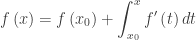
Notice that this is an accumulation function equation (Type 1).
  • Initial value differential equation problems: given the velocity or acceleration with initial condition(s) find the position or velocity. These are easily handled with the accumulation equation in the bullet above.
  • Find the speed at a given time. The speed is the absolute value of the velocity.
  • Find average speed, velocity, or acceleration
  • Determine if the speed is increasing or decreasing.
  • If at some time, the velocity and acceleration have the same sign then the speed is increasing.If they have different signs the speed is decreasing.
  • If the velocity graph is moving away from (towards) the t-axis the speed is increasing (decreasing).
  • See my post for November 19, 2012.
  • Use a difference quotient to approximate derivative.
  • Riemann sum approximations.
  • Units of measure.
  • Interpret meaning of a derivative or a definite integral in context of the problem

Shorter questions on this concept appear in the multiple-choice sections. As always, look over as many questions of this kind from past exams as you can find.

For some previous posts on this subject see November 1619, 2012, January 21, 2013. There is also a worksheet on speed here and on the Resources pages (click at the top of this page).

The BC topic of motion in a plane, (Type 8: parametric equations and vectors) will be discussed in a later post.


Next Posts:

Friday March 10: Graph Analysis (Type 3)

Tuesday March 14: Area and Volume (Type 4)

Friday March 17: Table and Riemann sums (Type 5)

Tuesday Match 21: Differential Equations (Type 6)

Friday March 24: Others (Type 7: related rates, implicit differentiation, etc.)


Rate and Accumulation Questions (Type 1)

The Free-response Questions

The free-response questions fall into 10 general categories or types. The multiple-choice questions fall largely into the same categories plus some straight-forward questions asking students to find limits, derivatives, and integrals. Often two or more type are combined into one question. The types are the following.

  1. Rate and Accumulation
  2. Linear motion
  3. Graph Analysis
  4. Area / Volume
  5. Table and Riemann sum
  6. Differential Equation (and slope fields)
  7. Others (implicit differentiation, related rates, theorems, et. al.)
  8. Parametric Equations (BC only)
  9. Polar Equations (BC only)
  10. Sequences and Series (BC only)

My numbering has changed over the years. This numbering follows this index where each type is referenced to free-response and multiple-choice questions of the same type.

I will discuss each type individually over the next few weeks starting today with Type 1.


AP Type Questions 1: Rate and Accumulation

These questions are often in context with a lot of words describing a situation in which some things are changing. There are usually two rates acting in opposite ways. Students are asked about the change that the rates produce over some time interval either separately or together.

The rates are often fairly complicated functions. If they are on the calculator allowed section, students should store the functions in the equation editor of their calculator and use their calculator to do any integration or differentiation that may be necessary.

The main idea is that integral of a rate of change over the time interval [a, b] is the net amount of change

\displaystyle \int_{a}^{b}{{f}'\left( t \right)dt}=f\left( b \right)-f\left( a \right)

If the question asks for an amount, look around for a rate to integrate.

The final (accumulated) amount is the initial amount plus the accumulated change:

\displaystyle f\left( x \right)=f\left( {{x}_{0}} \right)+\int_{{{x}_{0}}}^{x}{{f}'\left( t \right)}\,dt,

where {{x}_{0}} is the initial time, and  f\left( {{x}_{0}} \right) is the initial amount. Since this is one of the main interpretations of the definite integral the concept may come up in a variety of situations.

What students should be able to do:

  • Be ready to read and apply; often these problems contain a lot of writing which needs to be carefully read.
  • Recognize that rate = derivative.
  • Recognize a rate from the units given without the words “rate” or “derivative.”
  • Find the change in an amount by integrating the rate. The integral of a rate of change gives the amount of change (FTC):

\displaystyle \int_{a}^{b}{{f}'\left( t \right)dt}=f\left( b \right)-f\left( a \right).

  • Find the final amount by adding the initial amount to the amount found by integrating the rate. If x={{x}_{0}} is the initial time, and f\left( {{x}_{0}} \right)  is the initial amount, then final accumulated amount is

\displaystyle f\left( x \right)=f\left( {{x}_{0}} \right)+\int_{{{x}_{0}}}^{x}{{f}'\left( t \right)}\,dt,

  • Understand the question. It is often not necessary to as much computation as it seems at first.
  • Use FTC to differentiate a function defined by an integral.
  • Explain the meaning of a derivative or its value in terms of the context of the problem.
  • Explain the meaning of a definite integral or its value in terms of the context of the problem. The explanation should contain (1) what it represents, (2) its units, and (3) how the limits of integration apply in context.
  • Store functions in their calculator recall them to do computations on their calculator.
  • If the rates are given in a table, be ready to approximate an integral using a Riemann sum or by trapezoids.
  • Do a max/min or increasing/decreasing analysis.

Shorter questions on this concept appear in the multiple-choice sections. As always, look over as many questions of this kind from past exams as you can find.


For some previous posts on this subject see January 2123, 2013. This post is revised from the post of March 1, 2013


Next Posts:

Tuesday March 7: Type 2 Linear Motion

Friday March 10: Type 3: Graph Analysis


The Writing Questions on the AP Exams

The goals of the AP Calculus program state that, “Students should be able to communicate mathematics and explain solutions to problems both verbally and in well written sentences.” For obvious reasons the verbal part cannot be tested on the exams; it is expected that you will do that in your class. The exams do require written answers to parts of several questions. The number of points riding on written explanations on recent exams is summarized in the table below.

 Year AB BC
2007 9 9
2008 7 8
2009 7 3
2010 7 7
2011 7 6
2012 9 7
2013 9 7
2014 6 3
2015 8 6
2016 6 6

The average is between 6 and 8 points each year with some years having 9. That’s the equivalent of a full question. So, this is something that should not be overlooked in teaching the course and in preparing for the exams. Start long before calculus; make writing part of the school’s math program.

That a written answer is expected is indicated by phrases such as:

  • Justify you answer
  • Explain your reasoning
  • Why?
  • Why not?
  • Give a reason for your answer
  • Explain the meaning of a definite integral in the context of the problem.
  • Explain the meaning of a derivative in the context of the problem.
  • Explain why an approximation overestimates or underestimates the actual value

How do you answer such a question? The short answer is to determine which theorem or definition applies and then show that the given situation specifically meets (or fails to meet) the hypotheses of the theorem or definition.

Explanations should be based on what is given in the problem or what the student has computed or derived from the given, and be based on a theorem or definition. Some more specific suggestions:

  • To show that a function is continuous show that the limit (or perhaps two one-sided limits) equals the value at the point. (See 2007 AB 6)
  • Increasing, decreasing, local extreme values, and concavity are all justified by reference to the function’s derivative. The table below shows what is required for the justifications. The items in the second column must be given (perhaps on a graph of the derivative) or must have been established by the student’s work.
Conclusion Establish that
y is increasing y’ > 0  (above the x-axis)
y is decreasing y’ < 0   (below the x-axis)
y has a local minimum y’ changes  – to + (crosses x-axis below to above) or {y}'=0\text{ and }{{y}'}'>0
y has a local maximum y’ changes + to –  (crosses x-axis above to below) or {y}'=0\text{ and }{{y}'}'<0
y is concave up y’ increasing  (going up to the right) or {{y}'}'>0
y is concave down y’ decreasing  (going down to the right) or {{y}'}'<0
y has point of inflection y’ extreme value  (high or low points) or {{y}'}' changes sign.
  •  Local extreme values may be justified by the First Derivative Test, the Second Derivative Test, or the Candidates’ Test. In each case the hypotheses must be shown to be true either in the given or by the student’s work.
  • Absolute Extreme Values may be justified by the same three tests (often the Candidates’ Test is the easiest), but here the student must consider the entire domain. This may be done (for a continuous function) by saying specifically that this is the only place where the derivative changes sign in the proper direction. (See the “quiz” below.)
  • Speed is increasing on intervals where the velocity and acceleration have the same sign; decreasing where they have different signs. (2013 AB 2 d)
  • To use the Mean Value Theorem state that the function is continuous and differentiable on the interval and show the computation of the slope between the endpoints of the interval. (2007 AB 3 b, 2103 AB3/BC3)
  • To use the Intermediate Value Theorem state that the function is continuous and show that the values at the endpoints bracket the value in question (2007 AB 3 a)
  • For L’Hôpital’s Rule state that the limit of the numerator and denominator are either both zero or both infinite. (2013 BC 5 a)
  • The meaning of a derivative should include the value and (1) what it is (the rate of change of …, velocity of …, slope of …), (2) the time it obtains this value, and (3) the units. (2012 AB1/BC1)
  • The meaning of a definite integral should include the value and (1) what the integral gives (amount, average value, change of position), (2) the units, and (3) what the limits of integration mean. One way of determining this is to remember the Fundamental Theorem of Calculus \displaystyle \int_{a}^{b}{{f}'\left( x \right)dx}=f\left( b \right)-f\left( a \right). The integral is the difference between whatever f represents at b and what it represents at a. (2009 AB 2 c, AB 3c, 2013 AB3/BC3 c)
  • To show that a theorem applies state and show that all its hypotheses are met. To show that a theorem does not apply show that at least one of the hypotheses is not true (be specific as to which one).
  • Overestimates or underestimates usually depend on the concavity between the two points used in the estimates.

A few other things to keep on mind:

  • Avoid pronouns. Pronouns need antecedents. “It’s increasing because it is positive on the interval” is not going to earn any points.
  • Avoid ambiguous references. Phrases such as “the graph”, “the derivative”, or “the slope” are unclear. When they see “the graph” readers are taught to ask “the graph of what?” Do not make them guess. Instead say “the graph of the derivative”, “the derivative of f”, or “the slope of the derivative.”
  • Answer the question. If the question is a yes or no then say “yes” or “no.” Every year students write great explanations but never clearly say whether they are justifying a “yes” or a “no.”
  • Don’t write too much. Usually a sentence or two is enough. If something extra is in the explanation and it is wrong, then the credit is not earned even though the rest of the explanation is great.

As always, look at the scoring standards from past exam and see how the justifications and explanations are worded. These make good templates for common justifications. Keep in mind that there are other correct ways to write the justifications.


QUIZ

Here is a quiz that can help your students learn how to write good explanations.

Let f\left( x \right)={{e}^{x}}\left( x-3 \right) for 0\le x\le 5.

Find the location of the minimum value of f(x). Justify your answer three different ways (without reference to each other).

Don’t tell your students the three ways – they should know that!

The minimum value occurs at x = 2. The three ways to justify this are the First Derivative Test, the Second Derivative Test and the Candidates’ Test (aka: the Closed Interval Test). Let them discuss and constructively criticize each other’s answers. As a class, compare and contrast the students’ answers.


Next Posts:

Friday March 3: Type 1 of the 10 type questions: Rate and Accumulation

Tuesday March 7: Type 2 Linear Motion

Friday March 10: Type 3: Graph Analysis


Revised from a post of March 9, 2015.