Applications of integrals, part 2: Volume problems

One of the major applications of integration is to find the volumes of various solid figures.

Volume of Solids with Regular Cross-sections  This is where to start with volume problems. After all, solids of revolution are just a special case of solids with regular cross-sections.

Volumes of Revolution

Subtract the Hole from the Whole and Does Simplifying Make Things Simpler?

Visualizing Solid Figures

Area and Volume (Type 4)  also Area and Volume Question review notes.

Why you Never Need Cylindrical Shells

Painting a Point


Applications of integrals, part 1: Areas & Average Value

Usually the first application of integration is to find the area bounded by a function and the x-axis, followed by finding the area between two functions. We begin with these problems

First some calculator hints

Graphing Integrals using a graphing calculator to graph functions defined by integrals

Graphing Calculator Use  and Definition Integrals – Exam considerations Suggestions for using a calculator efficiently in area/volume problems

Area Problems

Area Between Curves

Under is a Long Way Down How to avoid “negative area.”

Density Functions Not often asked on the AP exams, but a good application related to area, nevertheless.

Who’d a thunk it? Some more complicated area problems for CAS solution.

Improper Integrals and Proper Areas – a BC topic

Average Value

Average Value of a Function

What’s a Mean Old Average Anyway – Discusses the different “average” in calculus

Half-full and Half Empty – Average Value

Average Value Activity to help students discover the Average Value formula


Who’d a thunk it?

Cubic Symmetry

Some things are fairly obvious. For example, if you look at the graphs of a few cubic equations, you might think that each is symmetric to a point and on closer inspection the point of symmetry is the point of inflection.

This is true and easy to prove. You can find the point of inflection, and then show that any point a certain distance horizontally on one side is the same distance above (or below) the point of inflection as a point the same distance horizontally on the other side is below (or above). Another way is to translate the cubic so that the point of inflection is at the origin and then show the resulting function is an odd function (i.e. symmetric to the origin).

But some other properties are not at all obvious. How someone thought to look for them is not even clear.

Tangent Line.

If you have cubic function with real roots of x = a, x = b, and x = c not necessarily distinct, if you draw a tangent line at a point where x is the average of any two roots, x = ½(a + b), , then this tangent line intersects the cubic on the x-axis at exactly the third root, x = c. Here is a Desmos graph illustrating this idea.

Here is a proof done with a CAS. The first line is a cubic expressed in terms of its roots.  The third line asks where the tangent line at x = m intersects the x-axis. The last line is the answer: x = c or whenever a = b (i.e. when the two roots are the same, in which case the tangent line is the x-axis and of course also contains x = c.

Areas
Even harder to believe is this: Draw a tangent line anywhere on a cubic. This tangent will intersect the cubic at a second point and the line and the cubic will define a region whose area is A1. From the second point draw a tangent what intersects the cubic at a third point and defines a region whose area is A2. The ratio of the areas A2/A1 = 16. I have no idea why this should be so, but it is.

Here is a proof, again by CAS: The last line marked with a square bullet is the computation of the ratio and the answer, 16, is in the lower right,

And if that’s not strange enough, inserting two vertical lines defines other regions whose areas are in the ratios shown in the figure below.

Who’d a thunk it?

.

Area & Volume (Type 4)

Given equations that define a region in the plane students are asked to find its area and the volume of the solid formed when the region is revolved around a line or used as a base of a solid with regular cross-sections. This standard application of the integral has appeared every year since 1969 on the AB exam and all but one year on the BC exam.

What students should be able to do:

  • Find the intersection(s) of the graphs and use them as limits of integration (calculator equation solving). Write the equation followed by the solution; showing work is not required. Usually no credit is earned until the solution is used in context (as a limit of integration). Students should know how to store and recall these values to save time and avoid copy errors.
  • Find the area of the region between the graph and the x-axis or between two graphs.
  • Find the volume when the region is revolved around a line, not necessarily an axis or an edge of the region, by the disk/washer method.
  • The cylindrical shell method will never be necessary for a question on the AP exams, but is eligible for full credit if properly used.
  • Find the volume of a solid with regular cross-sections whose base is the region between the curves. For an interesting variation on this idea see 2009 AB 4(b)
  • Find the equation of a vertical line that divides the region in half (area or volume). This involves setting up and solving an integral equation where the limit is the variable for which the equation is solved.
  • For BC only – find the area of a region bounded by polar curves: A=\tfrac{1}{2}\int\limits_{{{\theta }_{1}}}^{{{\theta }_{2}}}{{{\left( r\left( \theta  \right) \right)}^{2}}}d\theta

If this question appears on the calculator active section, it is expected that the definite integrals will be evaluated on a calculator. Students should write the definite integral with limits on their paper and put its value after it.  It is not required to give the antiderivative and if a student gives an incorrect antiderivative they will lose credit even if the final answer is (somehow) correct.

There is a calculator program available that will give the set-up and not just the answer so recently this question has been on the no calculator allowed section. (The good news is that in this case the integrals will be easy or they will be set-up-but-do-not-integrate questions.)

Occasionally, other type questions have been included as a part of this question. See 2016 AB5/BC5 which included an average value question and a related rate question along with finding the volume.

Shorter questions on this concept appear in the multiple-choice sections. As always, look over as many questions of this kind from past exams as you can find.

For some previous posts on this subject see January 911, 2013


Next Posts:

Friday March 17: Table and Riemann sums (Type 5)

Tuesday Match 21: Differential Equations (Type 6)

Friday March 24: Others (Type 7: related rates, implicit differentiation, etc.)

Tuesday March 28: for BC Parametric Equation (Type 8)


Rate and Accumulation Questions (Type 1)

The Free-response Questions

The free-response questions fall into 10 general categories or types. The multiple-choice questions fall largely into the same categories plus some straight-forward questions asking students to find limits, derivatives, and integrals. Often two or more type are combined into one question. The types are the following.

  1. Rate and Accumulation
  2. Linear motion
  3. Graph Analysis
  4. Area / Volume
  5. Table and Riemann sum
  6. Differential Equation (and slope fields)
  7. Others (implicit differentiation, related rates, theorems, et. al.)
  8. Parametric Equations (BC only)
  9. Polar Equations (BC only)
  10. Sequences and Series (BC only)

My numbering has changed over the years. This numbering follows this index where each type is referenced to free-response and multiple-choice questions of the same type.

I will discuss each type individually over the next few weeks starting today with Type 1.


AP Type Questions 1: Rate and Accumulation

These questions are often in context with a lot of words describing a situation in which some things are changing. There are usually two rates acting in opposite ways. Students are asked about the change that the rates produce over some time interval either separately or together.

The rates are often fairly complicated functions. If they are on the calculator allowed section, students should store the functions in the equation editor of their calculator and use their calculator to do any integration or differentiation that may be necessary.

The main idea is that integral of a rate of change over the time interval [a, b] is the net amount of change

\displaystyle \int_{a}^{b}{{f}'\left( t \right)dt}=f\left( b \right)-f\left( a \right)

If the question asks for an amount, look around for a rate to integrate.

The final (accumulated) amount is the initial amount plus the accumulated change:

\displaystyle f\left( x \right)=f\left( {{x}_{0}} \right)+\int_{{{x}_{0}}}^{x}{{f}'\left( t \right)}\,dt,

where {{x}_{0}} is the initial time, and  f\left( {{x}_{0}} \right) is the initial amount. Since this is one of the main interpretations of the definite integral the concept may come up in a variety of situations.

What students should be able to do:

  • Be ready to read and apply; often these problems contain a lot of writing which needs to be carefully read.
  • Recognize that rate = derivative.
  • Recognize a rate from the units given without the words “rate” or “derivative.”
  • Find the change in an amount by integrating the rate. The integral of a rate of change gives the amount of change (FTC):

\displaystyle \int_{a}^{b}{{f}'\left( t \right)dt}=f\left( b \right)-f\left( a \right).

  • Find the final amount by adding the initial amount to the amount found by integrating the rate. If x={{x}_{0}} is the initial time, and f\left( {{x}_{0}} \right)  is the initial amount, then final accumulated amount is

\displaystyle f\left( x \right)=f\left( {{x}_{0}} \right)+\int_{{{x}_{0}}}^{x}{{f}'\left( t \right)}\,dt,

  • Understand the question. It is often not necessary to as much computation as it seems at first.
  • Use FTC to differentiate a function defined by an integral.
  • Explain the meaning of a derivative or its value in terms of the context of the problem.
  • Explain the meaning of a definite integral or its value in terms of the context of the problem. The explanation should contain (1) what it represents, (2) its units, and (3) how the limits of integration apply in context.
  • Store functions in their calculator recall them to do computations on their calculator.
  • If the rates are given in a table, be ready to approximate an integral using a Riemann sum or by trapezoids.
  • Do a max/min or increasing/decreasing analysis.

Shorter questions on this concept appear in the multiple-choice sections. As always, look over as many questions of this kind from past exams as you can find.


For some previous posts on this subject see January 2123, 2013. This post is revised from the post of March 1, 2013


Next Posts:

Tuesday March 7: Type 2 Linear Motion

Friday March 10: Type 3: Graph Analysis


Density Functions

Density, as an application of integration, has snuck onto the exams. It is specifically not mentioned in the “Curriculum Framework” chapter of the 2016 Course and Exam Description, there is one example in the 2020 CED There is an example (#12 p. 58) in the AB sample exam question section of 2020 Course and Exam Description. The first time this topic appeared was in the 2008 AB Calculus exam. There was a hint in the few years before that with a question in the old Course Description book. Both questions will be discussed below. The idea is that students are supposed to understand integration well enough to apply their knowledge to a new situation (density). 

The Mathematics

A density function gives the amount of something per unit of length, area, or volume, for example

  • The density of a metal rod may be given in units of grams per centimeter.
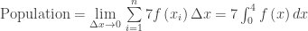
  • The density of the population of a city may be given in units of people per square mile. (See map at end.)
  • The density of a container of substance may be given in pounds per cubic foot.

The density can be used to find the amount. In each example, notice that the length, area, or volume of the region is multiplied by the density to find the amount.

Example 1: A 10 cm rod with a constant density of 3 g/cm has a mass of 10\text{ cm}\cdot \frac{3\text{ grams}}{\text{cm}}=30\text{ grams}

In other situations, the density is not constant and is given by some function. Suppose our metal rod of length b has a density of \rho \left( x \right) grams/cm where x is measured from one end of the rod. To find the total mass we think of cutting the rod in the very small pieces. (Think partition: each piece has a length of \Delta x in which the density is nearly constant say \rho \left( x \right).) The sum of the mass of these pieces is the Riemann sum \sum\limits_{i=1}^{n}{\rho \left( {{x}_{i}} \right)\Delta x}. The limit of this expression as \Delta x\to 0 gives the total mass in grams:
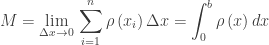
 \displaystyle M=\underset{\Delta x\to 0}{\mathop{\lim }}\,\sum\limits_{i=1}^{n}{\rho \left( {{x}_{i}} \right)\Delta x}=\int_{0}^{b}{\rho \left( x \right)dx} Notice that \sum\limits_{i=1}^{n}{\Delta x} is the length of the rod. This is multiplied by the density to find the mass.

Example 2: The next example is from the old Course Description book.

A city is built around a circular lake that has a radius of 1 mile. The population density of the city is f\left( r \right) people per square mile, where r is the distance from the center of the lake, in miles. Which of the following expressions gives the number of people who live within 1 mile of the lake?

(A) 2\pi \int_{0}^{1}{rf\left( r \right)dr}                 (B) 2\pi \int_{0}^{1}{r\left( 1+f\left( r \right) \right)dr}

(C) 2\pi \int_{0}^{2}{r\left( 1+f\left( r \right) \right)dr}      (D) 2\pi \int_{1}^{2}{rf\left( r \right)dr}

(E) 2\pi \int_{1}^{2}{r\left( 1+f\left( r \right) \right)dr}

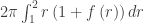
We need to partition the region so that each piece has a close to a constant density. Thin rings around the lake will accomplish this. A ring, if straightened out is similar to a rectangle of length 2\pi {{r}_{i}} where {{r}_{i}} is the distance from the center of the lake (this is the circumference of the ring), the width of this ring (rectangle) is \Delta r. In this ring (rectangle) the population density is people per square mile, so the population in the ring is f\left( {{r}_{i}} \right) approximated by multiplying the area by the density: 2\pi {{r}_{i}}f\left( {{r}_{i}} \right)\Delta r. Adding these gives a Riemann sum whose limit gives the total population:

\underset{\Delta x\to 0}{\mathop{\lim }}\,\sum\limits_{i=1}^{n}{2\pi {{r}_{i}}f\left( {{r}_{i}} \right)\Delta r}=2\pi \int_{1}^{2}{rf\left( r \right)dr}        Answer (D).

The limits of integration are from the edge of the lake, r = 1 to r = 2 (“one mile from the lake”). Another way to look at this is that \sum\limits_{i=1}^{n}{2\pi {{r}_{i}}\Delta r} is the area of the city; this is multiplied by the population density to find the population.

This type of density situation is called a radial density function.

Notice that the answer looks like the formula for volume by cylindrical shells; this is not quite an accident. The rings around the center are like the shells used when finding volume. It is the units that are different.

Example 3: From the 2008 AB Calculus exam #92.

density

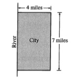
A city located beside a river has a rectangular boundary as shown in the figure above. The population density of the city at any point along a strip x miles from the river’s edge is f\left( x \right) people per square mile. Which of the following expressions gives the population of the city?

(A) \int_{0}^{4}{f\left( x \right)dx}          (B) 7\int_{0}^{4}{f\left( x \right)dx}          (C) 28\int_{0}^{4}{f\left( x \right)dx}

(D) \int_{0}^{7}{f\left( x \right)dx}          (E) 4\int_{0}^{7}{f\left( x \right)dx}

A thin vertical strip of the city {{x}_{i}} miles to the right of the river has an area of 7\Delta x. The population in each such strip is found by multiplying the area by the density function; this gives 7f\left( {{x}_{i}} \right)\Delta x. These are then added forming a Riemann sum, etc.

\text{Population}=\underset{\Delta x\to 0}{\mathop{\lim }}\,\sum\limits_{i=1}^{n}{7f\left( {{x}_{i}} \right)\Delta x}=7\int_{0}^{4}{f\left( x \right)dx}         Answer (B)

Alternative solution: When I first saw this question, not having thought about density for quite a while, I answered it by doing a unit analysis. Since unit analysis is a good thing for students to understand I’ll outline my thinking next.

We are looking for the population so the answer must be in units of “people.” The density function is in units of “people/square mile” (given). Both x and dx are in units of “miles” and the “7” also has units of “miles.” Therefore, the only choice that gives “people” is the one that multiplies the 7, the dx and the density function. This eliminates (A) and (D). The 28 in (C) must be square miles, making the overall units “people-miles” which is not what we’re going for. Finally, choice (E) is eliminated since the 7 and the dx are not in the same direction. This leaves (B).

Example 4: A volume problem adapted from Calculus by Hughes-Hallett, Gleason, et al.

The density of air h meters above the earth’s surface is \rho \left( h \right)=1.25{{e}^{-0.00012h}}\text{ kg/}{{\text{m}}^{3}}. Find the mass of a column of air 25 km high with a square base 3 meters on a side sitting on the surface of the earth.

At any height,  h meters above the earth the volume of a thin slice of the column of air is {{3}^{2}}\Delta h. The mass of this slice is {{3}^{2}}\rho \left( {{h}_{i}} \right)\Delta h. The sum of these slices gives a Riemann sum whose limit gives the total volume:

\displaystyle M=\underset{\Delta h\to 0}{\mathop{\lim }}\,\sum\limits_{i=1}^{n}{9\rho \left( {{h}_{i}} \right)\Delta h}=9\int_{0}^{25,000}{1.25{{e}^{-0.00012h}}dh}\approx 89,082\text{ kg}\text{.}


For other examples see 2018 BC 2, and 2021 AB 1, Good Question 15 and Good Question 16


Check the index of your textbook for density problems. Calculus by Hughes-Hallett Gleason, et al and Calculus by Rogawski (2nd edition) have good exercises and examples. My advice is not to make too big a deal of this, but if you have time, you can take a look. Should this kind of question appear on the free-response section I would guess that the question will be carefully worded so that students who never saw this kind of question would have a good chance of answering it.


The changing population density of Sydney, Australia in persons per hectare. Note the date changes in the key at the lower left.

sydney-density-1991-2011


Revised and updated 8-20-2019


Coming soon:

  • Jan 17th, Every Day series
  • Jan 24th, Logistic Growth – Real and Simulated
  • Jan 31st, The Logistic Equation
  • Feb 7th, Graphing Taylor Polynomials
  • Feb 14th,  Geometric Series – Far Out

Definite integrals – Exam Considerations

The sixth in the Graphing Calculator / Technology Series

Both graphing calculators and CAS calculators allow students to evaluate definite integrals. In the sections of the AP Calculus that allow calculator use students are expected to use their calculator to evaluate definite integrals. On the free-response section, students should write the integral on their paper, including the limits of integration, and then find its value on their calculator. There is no need to show the antiderivative; in fact, the antiderivative may be too difficult to find.

There are a few things students should be aware of. A question typically is worth three points: one point for the limits of integration and any constant (such as \pi in a volume problem), one point for the integrand, and one point for the numerical answer. An answer alone, with no integral, may not earn any points even if it is correct.

The “Instructions” on the cover of the free-response sections read “Show your work. … Your work will be scored on the correctness and completeness of your methods as well as your answers. Answers without supporting work will usually not receive credit.” [Emphasis added] The work must be on the paper, not just on the calculator.

Another consideration is accuracy. The general directions also say, “If you use decimal approximations in calculations, your work will be scored on accuracy. Unless otherwise specified, your final answers should be accurate to three places after the decimal point.”

Let’s see how all this works in an example.

Find the area of the region between the graphs of f\left( x \right)=x+3\cos (x) and g\left( x \right)={{\left( x-2 \right)}^{2}}. Begin by graphing the functions and finding their points of intersections on your graphing calculator.

integrals-3

The values are A = 0.22532 and B = 2.41524 (or 2.41525). Students should also store these values in their calculator and recall them for the computation, as explained in a previous post. Students should write these on their paper just as shown here. Notice that a few extra decimal places should be included.  The student should then show the integral and limits along with the answer on their paper:

\displaystyle \int_{A}^{B}{\left( x-3\cos \left( x \right)-{{\left( x-2 \right)}^{2}} \right)dx=2.32651}

Notice: Students may write A and B as the limits of integration, provided they have stated their values on the paper. This is best, but they may also write:

\displaystyle \int_{0.22532}^{2.41525}{\left( x-3\cos \left( x \right)-{{\left( x-2 \right)}^{2}} \right)dx=2.32651}

or even \displaystyle  \int_{0.225}^{2,415}{\left( x-3\cos \left( x \right)-{{\left( x-2 \right)}^{2}} \right)dx=2.32651}

But be careful!!! The unrounded values should be used to do the computation. Since the limits are answers they may be rounded, but if the rounding causes the final answer to not be accurate to three places past the decimal point, then the final answer is wrong, and the answer point will not be awarded. This has happened in the past. The safest thing is to use 5 or more decimal places in your computations.

Notice also that the final answer need not be rounded as long as the first three decimal places are correct.

.