
What is the probability that a triangle picked at random will be acute? An average value problem.
The thing here is to define what you mean by picking a triangle “at random.” You could open a Geometry book and take the first triangle you come to, but are the triangles in a Geometry book really a good sample space? I doubt it.
Let’s try this: let A, B, and C be the measures, in degrees, of the angles of 
Then

For any A < 90, B and C are chosen from the interval 
![[90-A,90]](https://s0.wp.com/latex.php?latex=%5B90-A%2C90%5D&bg=ffffff&fg=333333&s=0&c=20201002)
This is an interval of length A and the probability of picking numbers, B and C, at random in this interval is 

In general 
This average is
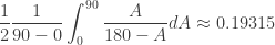
So about 19.3% of triangles are acute, the rest are obtuse (or right). Leaving one to believe that most triangles are obtuse.
Challenge: Try writing a calculator or computer program that picks the measures of the angles of a triangle as described above. Repeat this many times while the program counts the number of acute triangles and the total number of triangles and finds their ratio. Does it come close to 19.3%?
_______________
This problem was posted on the AP Calculus Electronic Discussion Group (11/22/03) by Stu Schwartz an AP Calculus teacher at Wissahickon High School in Ambler, Pennsylvania. The solution is by one of Mr. Schwartz’s students Kurt Schneider, a tenth grader at the time who completed AB calculus in eighth grade and BC calculus in ninth grade!
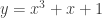
![\left[ 0,2\pi \right]](https://s0.wp.com/latex.php?latex=%5Cleft%5B+0%2C2%5Cpi+%5Cright%5D&bg=ffffff&fg=333333&s=0&c=20201002) and some others. The average appears to be 2, again since half the values are above and half below 2.
and some others. The average appears to be 2, again since half the values are above and half below 2.
 , and the lines y = 1 and x = 2, is revolved around the y-axis. What is the volume of the resulting solid?
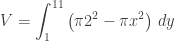

 , as the shell integral.
 from x = 0 to
 ; the thickness is
 .
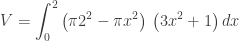
. ) from the outside volume (radius =
  ). This may be done with two integrals or combined into one.
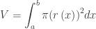
 is often factored out in front of the integral sign to make things look neater; I suggest you leave it where it is to remind students that they are subtracting the areas of two circles.
 .
.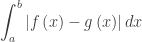 .
. . This is correct only if f (x) > 0. There is a natural confusion for beginning students between the facts that if f (x) < 0 the integral comes out negative, but the area is positive.
 which is positive as it should be. And students will immediately see that