
You have learned and used formulas for finding the derivatives of the Elementary Functions. These can be applied to functions made up of the Elementary Functions and extended to other expressions.
Many functions are made by combining the Elementary Functions. For example, polynomials are the sum and differences of a constants and powers of x multiplied by constants (their coefficients).
The functions you will look at next are the sums, differences, products, quotients, and/or composites of the Elementary Function. You will learn five techniques for handling these.
Sums and differences are found by differentiating the individual terms. Then there are the Product Rule for products of functions, the Quotient Rule for quotients and the Chain Rule for compositions. The techniques are often used in combinations.
Learn to see the patterns in the functions and learn what procedure to use for each.
HINT: Memorize the techniques as you learn them. After all these years, I still say the formulas and techniques as I use them. So, for products I repeat in my mind “the first times the derivative of the second plus the second times the derivative of the first” as I do the computation. Forget about mnemonics – just say the technique as you use it, and you’ll memorize it easily.
Implicit relations and inverses have their own techniques; they use the basic formulas and techniques in different ways.
Since derivatives are functions, they have their own derivatives. The derivative of the first derivative is called the second derivative. Then there is the third derivative, the fourth derivative and so on. Mostly, you will use only the first three. No new rules to learn; higher order derivatives are computed the same way as the first derivative, and in fact, they often get simpler.
The proofs of the formulas and techniques (they are really theorems) are interesting from a mathematical point of view. You should follow along when your teacher shows them to you so that you understand why they work and where they come from. You will not be asked to reproduce the proofs on the AP Calculus Exam.
AP Calculus Course and Exam Description Unit 3 Sections 2.8 – 2.10 and Unit 3 all
 where the point is
  and the slope is the derivative denoted by
  . You only need these three numbers – the two coordinates of a point and the derivative at that point). Drop them into the point-slope equation and you’re done.)
 , then
  and
and  .
. . Velocity has direction (indicated by its sign) and magnitude. Technically, velocity is a vector; the term “vector” will not appear on the AB exam.
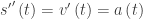 It, too, has direction and magnitude and is a vector.
 .
.
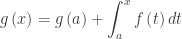
 Notice that this is an accumulation function equation (Type 1).
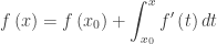
 is the initial time, and
  is the initial amount. Since this is one of the main interpretations of the definite integral the concept may come up in a variety of situations.