Implicit Differentiation

I discovered in doing next week’s post that I apparently never wrote about implicit differentiation. So here goes – an extra post this week!

Implicit Differentiation

The technique of implicit differentiation allows you to find slopes of relations given by equations that are not written as functions or may even be impossible to write as functions.

Example 1: A good way to start investigating this idea is to give your class the equation of a circle, say {{x}^{2}}+{{y}^{2}}=25 and ask them to find the slope of the tangent line (the derivative) where x = 3. No hints, just let them try.

Most students will hit upon solving for y and then differentiating:

y=\pm \sqrt{{25-{{x}^{2}}}}

\displaystyle \frac{{dy}}{{dx}}=\frac{{-2x}}{{\pm 2\sqrt{{25-{{x}^{2}}}}}}=\frac{{-x}}{{\pm \sqrt{{25-{{x}^{2}}}}}}

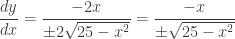
There are two points where x = 3: (3, 4) and (3, –4) at the first point the slope is – ¾ and at the second ¾.

Then show them another way – implicit differentiation.

To use this technique, assume that y is a function of x, but do not bother to find that function. Then using the chain rule on any terms containing a y. For{{x}^{2}}+{{y}^{2}}=25 , we have

\displaystyle 2x+2y\frac{{dy}}{{dx}}=0

Then solve for the derivative

\displaystyle \frac{{dy}}{{dx}}=-\frac{x}{y}

We see that this is the same as we found the first time, since y=\pm \sqrt{{25-{{x}^{2}}}}! There is a slight advantage here: we can now find the slopes from the coordinates without solving or dealing with the plus/minus sign. *

Example 2: Now let’s consider a more difficult example. Find the derivative of {{x}^{2}}+4{{y}^{2}}=7+3xy. To solve for y here is possible but somewhat difficult (Hint: use the quadratic formula). We can continue writing {y}' for dy/dx.

2x+8y{y}'=0+3x{y}'+3y

Note that the last term on the right is differentiated using the product rule.  Since this happens fairly often, students need to be reminded of it.

Now solving for {y}'gives

\displaystyle {y}'=\frac{{3y-2x}}{{8y-3x}}

Then we can find the derivatives at specific points by substituting the coordinates of the point. At the point (3,2) on the curve, the slope is \displaystyle {y}'=\frac{{3\left( 2 \right)-2\left( 3 \right)}}{{8\left( 2 \right)-3\left( 3 \right)}}=\frac{0}{7}=0

Note: the derivative of an implicit relation usually involves both the x and y coordinates.

Second Derivatives

This idea can be repeated to find second and higher derivatives.

Example 1 continued: In the first example with \displaystyle \frac{{dy}}{{dx}}=\frac{{-x}}{y}  we differentiate using the quotient rule:

\displaystyle  {{y}'}'=\frac{{y(-1)-(-x){y}'}}{{{{y}^{2}}}}

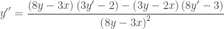
The second derivative is a function, not just of x and y, but also of {y}'. We can replace it with the first derivative and simplify.

\displaystyle  {{y}'}'=\frac{{-y+x\left( {\frac{{-x}}{y}} \right)}}{{{{y}^{2}}}}=\frac{{-{{y}^{2}}-{{x}^{2}}}}{{{{y}^{3}}}}=-\frac{{25}}{{{{y}^{3}}}}

(This might be a good time to do a quick review of simplifying complex fractions; they occur often in implicit differentiation problems.)

To find the value of the second derivative at a given point we can substitute into either of the two expressions above. At (3, –4) where the derivative has been previously found to be ¾ we have \displaystyle  {{y}'}'=\frac{{y(-1)-(-x){y}'}}{{{{y}^{2}}}}=\frac{{\left( {-4} \right)\left( {-1} \right)-\left( {-3} \right)\left( {\frac{3}{{-4}}} \right)}}{{{{{\left( {-4} \right)}}^{2}}}}=-\frac{{-16-9}}{{-48}}=\frac{{25}}{{48}}

Or we can use the second form

\displaystyle {{y}'}'=-\frac{{25}}{{{{y}^{3}}}}=-\frac{{25}}{{{{{\left( {-4} \right)}}^{3}}}}=\frac{{25}}{{48}}

Example 2 continued: The second example was taken from an AB Calculus exam (2004 AB 4). The first part gave the first derivative and asked students to show that it was correct. This was done (instead of just asking the students to find the first derivative) so that students would be sure to have the correct derivative to use later in the question.

The second part asked students to show that the tangent line is horizontal at the point where x = 3. This included finding the coordinates of the point, (3, 2) and showing that it is on the curve.

The third part of the question asked students to determine whether the point from part (b) was a relative maximum, a relative minimum or neither, and to justify their answer. Since there is no way to determine how the sign of the first derivative changes at the point the First Derivative Test cannot be used. Likewise, the Candidates’ Test (a/k/a the closed interval test) cannot be used without solving for y, and determining the domain of each part. That leaves the Second Derivative Test as the easiest choice.

\displaystyle {y}'=\frac{{3y-2x}}{{8y-3x}}  at (3,2) \displaystyle {y}'=\frac{{3\left( 2 \right)-2\left( 3 \right)}}{{8\left( 2 \right)-3\left( 3 \right)}}=0

\displaystyle {{y}'}'=\frac{{\left( {8y-3x} \right)\left( {3{y}'-2} \right)-\left( {3y-2x} \right)\left( {8{y}'-3} \right)}}{{{{{\left( {8y-3x} \right)}}^{2}}}}

Substituting the values into this without doing the algebra to remove the first derivative gives

\displaystyle \begin{array}{l}{{y}'}'=\frac{{\left( {8\left( 2 \right)-3\left( 3 \right)} \right)\left( {0-2} \right)-\left( {3\left( 2 \right)-2\left( 3 \right)} \right)\left( {8\left( 0 \right)-3} \right)}}{{{{{\left( {8\left( 2 \right)-3\left( 3 \right)} \right)}}^{2}}}}=\frac{{\left( {16-9} \right)\left( {-2} \right)-0}}{{{{{\left( {16-9} \right)}}^{2}}}}=-\frac{2}{7}\\\end{array}

So, the point (3, 2) is a relative maximum.

The graph of the relation, an ellipse is shown below.


* Incidentally, there is another clever way of doing example 1: The radius to any point on a circle centered at the origin has a slope of y/x.  Since tangents to circles are perpendicular to the radii drawn to the point of tangency, the slope of the tangent must be –x/y.


The Chain Rule

Most of the function students are faced with in beginning calculus are compositions of the Elementary Functions. The Chain Rule allows you to differentiate composite functions easily. The posted listed below are ways to introduce and then use the Chain Rule.

Experimenting with a CAS – Chain Rule  Using a CAS to discover the Chain Rule

Power Rule Implies Chain Rule and Foreshadowing the Chain Rule the same ideas.

The Chain Rule


Differentiation Techniques

Maria Gaetana Agnesi

So, no one wants to do complicated limits to find derivatives. There are easier ways of course. There are a number of quick ways (rules, formulas) for finding derivatives of the Elementary Functions and their compositions. Here are some ways to introduce these rules; these are the subject of this week’s review of past posts.

Why Radians?

The Derivative I        Guessing the derivatives from the definition

The Derivative II      Using difference Quotient to graph and guess

The Derivative Rules I    The Power Rule

The Derivative Rules II       Another approach to the Product Rule from my friend Paul Foerster

The Derivative Rules III     The Quotient Rule developed using the Power Rule, an approach first suggested  by Maria Gaetana Agnesi (1718 – 1799) who was helping her brother learn the calculus.

Next week: The Chain Rule.


Difference Quotients

Difference quotients are the path to the definition of the derivative. Here are three posts exploring difference quotients.

Difference Quotients I  The forward and backward difference quotients

Difference Quotients II      The symmetric difference quotient and seeing the three difference quotients in action.  Showing that the three difference quotients converge to the same value.

Seeing Difference Quotients      Expands on the post immediately above and shows some numerical and graphical approaches using calculators and Desmos.

 Tangents and Slopes You can use this Desmos app now to preview some of the things that he tangent line can tell us about the graph of a function or save (or reuse) it for later when concentrating on graphs. Discuss slope in relation to increasing, decreasing, concavity, etc.

At Just the Right Time

Stamp out Slope-intercept Form


Working up to the derivative.

While limit is what makes all of the calculus work, people usually think of calculus as starting with the derivative. The first problem in calculus is finding the slope of a line tangent to a graph at a point and then writing the equation of that tangent line.

Local Linearity is the graphical manifestation of differentiability. If you zoom-in of the graph of a function (at a point where we will soon say the function is differentiable), the graph eventually looks like a line: the graph appears to be straight, and its slope is the number we will call its derivative.

To do this we need to zoom-in numerically. Zooming-in numerically is accomplished by finding the slope of a secant line, a line that intersects the graph twice, and then finding the limit of that slope as the two points come closer together.

This week’s posts start with local linearity and tangent lines. They lead to the difference quotient and the equation of the tangent line.

Local Linearity I

Local Linearity II      Working up to difference quotient. The next post explains this in more detail.

Tangent Lines approaching difference quotients on calculator by graphing tan line.

Next week: Difference Quotients.


Who’d a thunk it?

Cubic Symmetry

Some things are fairly obvious. For example, if you look at the graphs of a few cubic equations, you might think that each is symmetric to a point and on closer inspection the point of symmetry is the point of inflection.

This is true and easy to prove. You can find the point of inflection, and then show that any point a certain distance horizontally on one side is the same distance above (or below) the point of inflection as a point the same distance horizontally on the other side is below (or above). Another way is to translate the cubic so that the point of inflection is at the origin and then show the resulting function is an odd function (i.e. symmetric to the origin).

But some other properties are not at all obvious. How someone thought to look for them is not even clear.

Tangent Line.

If you have cubic function with real roots of x = a, x = b, and x = c not necessarily distinct, if you draw a tangent line at a point where x is the average of any two roots, x = ½(a + b), , then this tangent line intersects the cubic on the x-axis at exactly the third root, x = c. Here is a Desmos graph illustrating this idea.

Here is a proof done with a CAS. The first line is a cubic expressed in terms of its roots.  The third line asks where the tangent line at x = m intersects the x-axis. The last line is the answer: x = c or whenever a = b (i.e. when the two roots are the same, in which case the tangent line is the x-axis and of course also contains x = c.

Areas
Even harder to believe is this: Draw a tangent line anywhere on a cubic. This tangent will intersect the cubic at a second point and the line and the cubic will define a region whose area is A1. From the second point draw a tangent what intersects the cubic at a third point and defines a region whose area is A2. The ratio of the areas A2/A1 = 16. I have no idea why this should be so, but it is.

Here is a proof, again by CAS: The last line marked with a square bullet is the computation of the ratio and the answer, 16, is in the lower right,

And if that’s not strange enough, inserting two vertical lines defines other regions whose areas are in the ratios shown in the figure below.

Who’d a thunk it?

.

Synthetic Summer Fun

Today, for some summer fun, let’s look at synthetic division a/k/a synthetic substitution. I’ll assume you all know how to do that since it is a pretty common pre-calculus topic and even comes up again in calculus.

Why Does Synthetic Division Work?

An example: consider the polynomial

P(x)=2{{x}^{4}}-3{{x}^{3}}-11{{x}^{2}}+14x-1.

This can be written in nested form like this

P(x)=((((2x-3)x-11)x+14)x-1)

To evaluate this last expression at, say x = 2, we do the arithmetic as follows:

  1.   2 x 2 – 3 = 1
  2.   2 x 1 – 11 = –9
  3.   2 x (–9) + 14 = –4
  4.   2 x (–4) – 1 = – 9 = f(2)

Notice that this requires only multiplication and addition or subtraction, no raising to powers. More to the point, this is the same arithmetic, in the same order when you do the evaluation by synthetic division, and the work is a little easier to keep track of.

\begin{matrix} {} & 2 & -3 & -11 & 14 & -1 \\ 2) & 2 & 1 & -9 & -4 & -9 \\ \end{matrix}\begin{matrix} {} \\ \,=P(2) \\ \end{matrix}

Synthetic division has another advantage: the other numbers in the second row are the coefficients of a quotient polynomial, a polynomial of one less degree that the original. So,

\displaystyle \frac{P(x)}{x-2}=2{{x}^{3}}+{{x}^{2}}-9x-4+\frac{-9}{x-2}

The Remainder Theorem and the Factor Theorem

In general, a polynomial of degree n, divided by a linear factor (x – a) gives a polynomial Q(x) of degree n – 1 and a remainder R

\displaystyle \frac{P(x)}{x-a}=Q(x)+\frac{R}{x-a}

Or

P(x)=Q(x)(x-a)+R

From here it is easy to see that P(a)=R
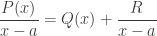
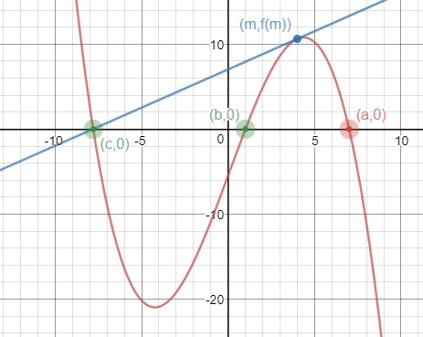
. This is called the remainder theorem. It has a corollary called the factor theorem: If R = 0, then (x – a) is a factor of P(x).

Calculus

But wait there is more: differentiating the equation above using the product rule gives

{P}'(x)=Q(x)(1)+Q(x)(x-a)+0 and substituting x = a  gives

{P}'(a)=Q(a). The value of the quotient polynomial at a is the derivative of the original polynomial at a.
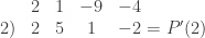
Of course, we could also rewrite the same equation as \displaystyle \frac{P(x)-P(a)}{x-a}=Q(x) . Then

\displaystyle {P}'(a)=\underset{x\to a}{\mathop{\lim }}\,\frac{P(x)-P(a)}{x-a}=\underset{x\to a}{\mathop{\lim }}\,Q(x)=Q(a)

Taylor Series

But wait, there’s even more.

A polynomial is a Maclaurin series in which all the terms after the nth term are zero. When you students are first learning how to write a Taylor series, by finding all the derivatives and substituting in the general term, a good exercise is to have them write the Taylor series for a polynomial centered away from the origin. For the example above:

P(x)=-9-2\left( x-2 \right)+19{{\left( x-2 \right)}^{2}}+13{{\left( x-2 \right)}^{3}}+2{{\left( x-2 \right)}^{4}}

Then ask them to expand the expression above and collect term etc. They should get the original polynomial again (and have some great practice expand powers of a binomial).

Can synthetic division help us? Yes, of course.  Here, is the original computation again:

\begin{matrix} {} & 2 & -3 & -11 & 14 & -1 \\ 2) & 2 & 1 & -9 & -4 & -9 \\ \end{matrix}\begin{matrix} {} \\ \,=P(2) \\ \end{matrix}

If we ignore the –9 and divide the quotient numbers by 2 we get

\begin{matrix} {} & 2 & 1 & -9 & -4 \\ 2) & 2 & 5 & 1 & -2 \\ \end{matrix}\begin{matrix} {} \\ \ ={P}'(2) \\ \end{matrix}

\begin{matrix} {} & 2 & 5 & 1 \\ 2) & 2 & 9 & 19 \\ \end{matrix}\begin{matrix} {} \\ \ =\frac{{{P}'}'(2)}{2} \\ \end{matrix}

And again

\begin{matrix} {} & 2 & 9 \\ 2) & 2 & 13 \\ \end{matrix}\begin{matrix} {} \\ \ =\frac{{{{P}'}'}'\left( 2 \right)}{3!} \\ \end{matrix}

One more time

\begin{matrix} {} & 2 \\ 2) & 2 \\ \end{matrix}\begin{matrix} {} \\ \ =\frac{{{P}^{(4)}}\left( 2 \right)}{4!} \\ \end{matrix}

What do you see? Right, the last numbers in each computation, –9, –2, 19, 13, and 2, are the coefficients of the Taylor polynomial!

If you really want to dive this home and have some more summer fun here’s the start of a proof (at least for n = 4). Let

P(x)={{c}_{4}}{{x}^{4}}+{{c}_{3}}{{x}^{3}}+{{c}_{2}}{{x}^{3}}+{{c}_{1}}x+{{c}_{0}} 
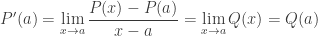
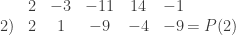
and divide this by a:

\begin{matrix} {} & {{c}_{4}} & {{c}_{3}} & {{c}_{2}} & {{c}_{1}} & {{c}_{0}} \\ a) & {{c}_{4}} & {{c}_{4}}a+{{c}_{3}} & {{c}_{4}}{{a}^{2}}{{+}_{{}}}{{c}_{3}}a+{{c}_{2}} & {{c}_{4}}{{a}^{3}}+{{c}_{3}}{{a}^{2}}+{{c}_{a}}a+{{c}_{1}} & {{c}_{4}}{{a}^{4}}+{{c}_{3}}{{a}^{3}}+{{c}_{a}}{{a}^{2}}+{{c}_{1}}a+{{c}_{0}}=P(a) \\ \end{matrix}

Again

\begin{matrix} {} & {{c}_{4}} & {{c}_{4}}a+{{c}_{3}} & {{c}_{4}}{{a}^{2}}{{+}_{{}}}{{c}_{3}}a+{{c}_{2}} & {{c}_{4}}{{a}^{3}}+{{c}_{3}}{{a}^{2}}+{{c}_{2}}a+{{c}_{1}} \\ a) & {{c}_{4}} & 2{{c}_{4}}a+{{c}_{3}} & 3{{c}_{4}}{{a}^{2}}+2{{c}_{3}}a+{{c}_{2}} & 4{{c}_{4}}{{a}^{3}}+3{{c}_{3}}{{a}^{2}}+2{{c}_{2}}a+{{c}_{1}} \\ \end{matrix}\begin{matrix} {} \\ \ ={P}'(a) \\ \end{matrix}

And I’ll leave the rest to you.  Really, why should I have all the fun?

.