I have mixed feelings about proof in high school math and high school calculus. I am not one for proving everything. For one thing, it cannot be done and, if it could be done, proof would become the whole focus of high school math. Proofs are not the focus of first-year calculus or AP calculus. The place for proving “everything” is a real analysis course in college.
However, students should know about proof and there are places where you can demonstrate some of the power of proof and show how proof works in calculus.
It is important, I think, that students know why a theorem is true; this helps in understanding what the theorem means. Some, but by no means all, proofs can show the student why the theorem is true. With other theorems there may be easier ways than a proof to convince someone of its truth.
In this and the next three posts, I propose to look at three theorems, the definitions used in them, and the ideas in their proofs. These are the theorems that lead up to the Mean Value Theorem (MVT). The MVT is a major result in calculus has many uses. Here goes:
Fermat’s theorem (not his famous “last” theorem, but an earlier one) says, that if a function is continuous on a closed interval and has a maximum (or minimum) value on that interval at x = c, then the derivative at x = c is either zero or does not exist.
The proof goes like this:
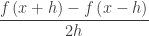
There are two cases. In each case we will look at the limit of the difference quotient that defines the derivative at x = c, namely,  and look at what happens as h approaches 0 from the left and from the right. These two limits are the same and equal to the derivative if, and only if, the derivative at c exists.
Also note that since we are assuming f(c) is a maximum, f (c) ≥ f (c + h) regardless of whether h is positive or negative. The numerator of the difference quotient is always zero or negative. Then if in the denominator h < 0, the quotient is non-positive; likewise, if h > 0, the quotient is non-negative.
Case I: The two limits are not equal. In this case the derivative does not exist. This could occur with a piecewise function, where two pieces with different derivatives meet at x = c.
Case II: The limits are equal. In this case the limit from the left (h < 0) must be greater than or equal to zero (since the function is increasing there) and the limit from the right (h > 0) must be less than or equal to zero. Then, the only way the limits can be equal is if both limits are zero; therefore the derivative is zero.
Any place where the derivative of a continuous function is zero or undefined is called a critical point and the number c is called a critical number (new definitions).
I think this proof is interesting because while there are lots of symbols flying around the key is interpreting what kind of number (positive, zero or negative) the symbols represent. Another thing I like is having to “read” the symbols and see that 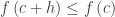 and therefore
The next post will discuss Rolle’s theorem.


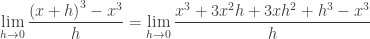
 . Most students will expand the binomial to get
  and differentiate the result to get
  . They will try the same approach with
  and then you can hit them with
  . They will see the need for a short cut at once. What to do?
 and let
  . Then our original expression becomes
 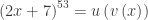 a composition of functions. The Chain Rule is used for differentiating compositions. Students must get good at recognizing compositions. The differentiation is done from the outside, working inward. It is done in the exact opposite order than the procedure for evaluating expression. To evaluate the expression above you (1) evaluate the expression inside the parentheses and the (2) raise that result to the 53 power. To differentiate you (1) use the power rule to differentiate the 53 power of whatever is inside, this gives
  , the (2) differentiate the
  which give 2 and multiply the results:
  . Symbolically, this looks like
  or
or  . This can be extended to compositions of more than two functions:
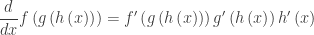

 . This function takes on all the values of
  in order in one-third the time. (That is its period is one-third of the period of
  .
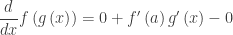
. , and let g be a function that is differentiable at
  and such that
  . Then, near
  :
:


 .
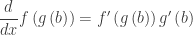
. and
and  .
. :
:

 and
and  . So now
  and
and  . Is this
  ? No it is not!
 ? How about the original functions?
 is hardly something you would expect anyone to figure out by themselves. As I mentioned, I’m more into explaining than proving.