Graphing Calculators

Posted on February 4, 2015 by Lin McMullin

I was asked to pass the following information along to you. I decided to do so because you may want to know about one of the newest CAS calculator models and because their follow-up offer for attending the summer institute is so generous. If your school and students need help getting calculators and/or you want to keep up with the latest trends, you may be interested in looking into this.

The calculator is the new Hewlett-Packard HP Prime. It is a CAS calculator with really good graphing features. HP is offering the HP Prime AP Summer Institute Program, a 3-Day Institute this summer in either Statistics or Calculus with expert teacher trainers to introduce their new Mathematics Solution, the HP Prime Wireless Classroom. Following the Summer Institute, teachers who attended will receive a donated HP Prime Wireless Classroom Kit for their school with 30 HP Prime Graphing Calculators and the HP Prime Wireless Kit (a $5,000 value!).

The institute is an opportunity to improve your knowledge of teaching mathematics with a technology that makes learning intuitive for students and receive the technology to keep for classroom use.

For more information click the link https://h30602.www3.hp.com/assets/hpmath/web1.html

Some Graphing Calculator History

Graphing calculators first came on the market around 1989. In the early 1990s after it was announced that graphing calculators would be required on the AP Calculus exams starting in 1995, there were a series of workshops following the AP calculus reading, then at Clemson University. They were called the Technology Intensive Calculus for Advanced Placement conference or TICAP. Half the readers were invited to stay after the reading for the conference. The next year the other half were invited, and others the third year. Casio, Texas Instruments, Hewlett-Packard, and Sharpe all contributed and provided their calculators to the participants.

The Texas Instrument calculators (then the TI-81 and TI-82) emerged the most popular and have since been the most popular in the United States. TI to their credit makes a good product and provided, and still provides, lots of help for teachers in the form of print material, programs for the calculators, workshops, and meetings. They have developed ways to connect the classroom’s calculators to the teacher’s computer. Other manufacturers have done the same, but not on TI’s scale.

TI has made improvements in their calculators and other manufacturers have made newer and improved machines as well. While similar in functionality, I think the Casio PRIZM to be a bit better than the latest TI-84 model; it is also a bit less expensive. TI’s ‘Nspire line is an excellent CAS machine. Casio also has several CAS calculators and HP has now come out with the new HP Prime model (mentioned above). There are others. TI has a whopping 92% market share with Casio far behind at 7%. While their machines are excellent, Casio and HP are playing catch-up and have a long way to go.

If you are just starting out or have limited funds for your class, you might consider a different brand. I often think the main problem is that the buttons are all in the wrong place! That is, the keyboards are different than the TIs we all learned on. They are different for you, but students who have never learned the old way will have no trouble with the keyboards. You won’t either – just sit down with the guidebook for a couple of hours and you’ll become an expert (or let the kids help you!). You can also use the manufacturer’s online instructions or go to a summer institute such as HP’s mentioned above.

Some Graphing Calculator Opinion

Now comes the real heresy. Graphing calculators don’t graph all that well. Their screens are small and often crowded. Tablets such as an iPad, or computers do a much better job. (For example, TI-Nspire’s operating system is available as an iPad app that is easy to use and much easier to see (okay maybe I’m getting old and my eyes are not what they once were). Still the many other graphing and mathematics related apps available are fabulous. Graphing, statistics and geometry apps abound and will only increase in number and functionality. This is the future.

The reason graphing calculators are still here is because the Educational Testing Service, for good reason, will not let students use any device with a QWERTY keyboard on their exams including the Advanced Placement exams. The primary reason is that they are afraid that students will copy the secure questions using the QWERTY keyboards on iPads and computers. For some reason, students apparently cannot figure out how to do this with the alphabetic keyboards on graphing calculators. (Or as Dan Kennedy once quipped, there is nothing wrong with the old method of writing them on your cuff.) Other more important reasons tablets are not allowed include being able to photograph the questions, get information and help through the internet during the exams, or communicating with others in or out of class with tweets and instant messages.

These are real problems that need to be considered, but I cannot believe a work-around is not possible. It must be possible to make an app that will allow only the use of approved apps during exams. After all they have done that for graphing calculators.

If technology helps students learn mathematics – and I believe it does – then students should have the best available technology.

End of sermon. Take a moment or more to consider the new and improved calculators.

Update – iPad’s “Educational Standardized Testing” Option

I wrote the paragraphs above a few days ago. This morning the new operating system 8.1.3 for iPad became available. They have a new feature for “educational standardized testing.” You can turn it on under Settings > Accessibility > Guided Access. Once turned on you open any app, triple-click the home button, and the controls for that one app appear on the screen.

The individual settings are slightly different for each app. You may turn off the keyboard, turn off the touch screen, or disable the dictionary. On apps with their own buttons you can turn off any or all of the buttons by circling them. A time limit may also be set.

It appears for now that each iPad must have these features adjusted individually. Unfortunately, to change or turn the restricted features on again all a student needs is his or her passcode or fingerprint. In addition, there should be a way to turn off all the other apps where students may quite legitimately have notes or homework saved. (Most of my students last year in one-to-one classrooms took most of their notes and did their homework on their iPads.)

This is a good start, but it has a long way to go before it can be used in group settings. Stay tuned for updates.

February 2015

Posted on February 1, 2015 by Lin McMullin

Calculus Teacher Makes the Big Times

Yitang Zhang

Photo by Peter Bohler – The New Yorker, February 2, 2015

Before turning to this month’s posts, I thought you might be interested in this. There is an interesting profile of Yitang Zhang in this week’s The New Yorker magazine by Alex Wilkinson. Mr. Zhang is a mathematician whose interest is “bound gaps” a problem in number theory on prime numbers. He is a part-time calculus teacher at the University of New Hampshire. He has won several prizes including a MacArthur award.

The profile is entitled The Pursuit if Beauty.

Wilkinson also made a short video explaining the “bound gaps” problem.

February

This month our previous posts finish a series on accumulation started in January and includes notes on power series. I have a few new post planned for February. Towards of the end of the month I plan to post a list of the previous posts on reviewing for the AP exams. As usual the four posts directly below are the most popular from previous Februarys. The most popular by a factor of about 50 (really) is the one on Error Bounds followed by iPads.

As always, please feel free to comment, question, or ask questions. I can use some suggestions about what you would like me to write about. My email address is lnmcmullin@aol.com. Notice, I’m a natural logarithm.

Thanks in advance.

Posts from past Februarys

February 2, 2013: Accumulation and Differential Equations Accumulation 6: Differential equations

February 4, 2013: Painting a Point Accumulation 7: An application (of paint)

February 8, 2013: Introducing Power Series 1

February 11, 2013: Introducing Power Series 2

February 13, 2013: Introducing Power Series 3

February 15, 2013 New Series from Old 1

February 18, 2013: New Series from Old 2

February 20, 2013: New Series from Old 3

February 22, 2013: Error Bounds

February 17, 2014 iPads

Good Question 1: 2008 AB 6

Posted on January 21, 2015 by Lin McMullin

When I started this blog several years ago I was hoping my readers would ask questions that we could discuss or submit ideas for additional topics to write about. This has not really happened, but I’m still very open to the idea. (That was a HINT.) Since that first year when I had the entire curriculum ahead of me, I have written less not because I dislike writing, but because I am low on ideas.

The other day, I answered a question posted on the AP Calculus Community bulletin board about AB calculus exam question. It occurred to me that this somewhat innocuous looking question was quite good. So I decided to start an occasional series on good questions, from AP exams or elsewhere, that can be used to teaching beyond the actual things asked in the question. (My last post might be in this category, but that was written several months ago.)

In discussing these questions, I will make numerous comments about the question and how to take it further in your class. My idea is not just to show how to write a good answer, but rather to use the question to look deeper into the concepts involved.

Good Question #1: 2008 AB Calculus exam question 6.

The stem gave students the function $\displaystyle f\left( x \right)=\frac{\ln \left( x \right)}{x},\quad x>0$ . Students were also told that $\displaystyle {f}'\left( x \right)=\frac{1-\ln \left( x \right)}{{{x}^{2}}}$ .

The first thought that occurs is why they gave the derivative. The reason is, as we will see, that the first derivative is necessary to answer the first three parts of the question. Therefore, a student who calculates an incorrect derivative is going to be in big trouble (and the readers may have a great deal of work to do reading with the student’s incorrect work). The derivative is calculated using the quotient rule, and students will have to demonstrate their knowledge of the quotient rule later in this question; there is no reason to ask them to do the same thing twice.
If you are using this with a class, you can, and probably should, ask your students to calculate the first derivative. Then you can see how many giving the derivative would have helped.
When discussing the stem, you should also discuss the domain, x > 0, and the x-intercept (1, 0). Other features of the graph, such as end behavior, are developed later in the question, so they may be put on hold briefly.

Part a asked students to write an equation of the tangent line at x = e². To do this students need to do two calculations: $\displaystyle f\left( {{e}^{2}} \right)=\frac{2}{{{e}^{2}}}$ and $\displaystyle {f}'\left( {{e}^{2}} \right)=-\frac{1}{{{e}^{4}}}$ . An equation of the tangent line is $\displaystyle y=\frac{2}{{{e}^{2}}}-\frac{1}{{{e}^{4}}}\left( x-{{e}^{2}} \right)$ .

Writing the equation of a tangent line is a very important skill and should be straightforward. The point-slope form is the way to go. Avoid slope-intercept.
The tangent line is used to approximate the value of the function near the point of tangency; you can throw in an approximation computation here.
After doing part c, you should return here and discuss whether the approximation is an overestimate or an underestimate and how you can tell. (Answer: underestimate, since the graph is concave up here.)
After doing part c, you can also ask them to write the tangent line at the point of inflection and whether approximations near the point of inflection are overestimates or an underestimates, and why. (Answer: Since the concavity change here, it depends on which side of the point of inflection the approximation is made. To the left is an overestimate; to the right is an underestimate.)

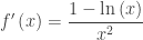Part b asked students to find the x-coordinate of the critical point, determine whether it is a maximum, a minimum, or neither, and to “justify your answer.” To earn credit students had to write the equation $\displaystyle {f}'\left( x \right)=0$ and solve it getting x = e. They had to state that this is a maximum because “ ${f}'\left( x \right)$ changes from positive to negative at x = e.”

This is a very standard AP exam question. To expand it in your class:

Discuss how you know the derivative changes sign here. This will get you into the properties of the natural logarithm function.
Discuss why the change in sign tells you this is a maximum. (A positive derivative indicates an increasing function, etc.)
After doing part c, you can return here and try the second derivative test.
The question asks for “the” critical point, hinting that there is only one. Students should learn to pick up on hints like this and be careful if their computation produces more or less than one.
At this point we have also determined that the function is increasing on the interval $\left( -\infty ,e \right]$ and decreasing everywhere else. The question does not ever ask this, but in class this is worth discussing as important features of the graph. On why these are half-open intervals look here.

Part c told students there was exactly one point of inflection and asked them to find its x-coordinate. To do this they had to use the quotient rule to find that $\displaystyle {{f}'}'\left( x \right)=\frac{-3+2\ln \left( x \right)}{{{x}^{3}}}$ , set this equal to zero and find the x-coordinate to be x = e^3/2.

The question did not require any justification for this answer. In class you should discuss what a justification would look like. The reason is that the second derivative changes sign here. So now you need to discuss how you know this.
Also, you can now determine that the function is concave down on the interval $\left( -\infty ,{{e}^{3/2}} \right)$ and concave up on the interval $\left({{e}^{3/2}},\infty \right)$ . Ask your class to justify this.

Part d asked student to find $\displaystyle \underset{x\to 0+}{\mathop{\lim }}\,\frac{\ln \left( x \right)}{x}$ . The answer is $-\infty$ . While this seems almost like a throwaway tacked on the end because they needed another point, it is the reason I like this question.

The question is easily solved: $\displaystyle \underset{x\to 0+}{\mathop{\lim }}\,\frac{\ln \left( x \right)}{x}=\underset{x\to 0+}{\mathop{\lim }}\,\frac{1}{x}\cdot \underset{x\to 0+}{\mathop{\lim }}\,\ln \left( x \right)=\left( \infty \right)\left( -\infty \right)=-\infty$ .
While tempting, the limit cannot be found by L’Hôpital’s Rule, because on substitution you get $\frac{-\infty }{0}$ ,which is not one of the forms that L’Hôpital’s Rule can handle.
The reason I like this part so much is that we have already developed enough information in the course of doing the problem to find this limit! The function is increasing and concave down on the interval $\left( -\infty ,e \right)$ . Moving from the maximum to the left, the function crosses the x-axis at (1, 0), keeps heading south, and gets steeper. So the limit as you approach the y-axis from the right is negative infinity.This is the left-side end behavior.
What about the right-side end behavior? (You ask your class.) Well, the function is positive and decreasing to the right of the maximum and becomes concave up after x = e^3/2. Thus, it must flatten out and approach the x-axis as an asymptote.
That $\displaystyle \underset{x\to \infty }{\mathop{\lim }}\,\frac{\ln \left( x \right)}{x}=0$ is clear from the note immediately above. This limit can be found by L’Hôpital’s Rule since it is an indeterminate of the type $\infty /\infty$ . So, $\displaystyle \underset{x\to \infty }{\mathop{\lim }}\,\frac{\ln \left( x \right)}{x}=\underset{x\to \infty }{\mathop{\lim }}\,\frac{\tfrac{1}{x}}{1}=0$ .
Notice also that the first derivative approaches zero as x approaches infinity. This indicates that the function’s graph approaches the horizontal as you travel farther to the right. The second derivative also approaches zero as x approaches infinity indicating that the function’s graph is becoming flatter (less concave).

This question and the discussion is largely done analytically (working with equations). We did find a few important numbers in the course of the work. Hopefully, you students discussed this with many good words. To complete the Rule of Four, here is the graph.

And here is a close up showing the important features of the graph and the corresponding points on the derivatives.

The function is shown in blue, the derivative and maximum in red, and the second derivative and the point of inflection in green.

Finally, this function and the limit at infinity is similar to the more pathological example discussed in the post of October 31, 2012 entitled Far Out!

Half-full and Half-empty

Posted on January 16, 2015 by Lin McMullin

A thought experiment:

Suppose you had a container with a rectangular base whose length runs from x = a to x = b, with a width of one inch. The container has four vertical rectangular sides. You put a piece of, say, plastic into the container which fits snugly along the bottom and four sides. The top of the piece is irregular and has the equation y = f(x). If the plastic were to melt, how high up the sides would the melted plastic rise?

One way to think about this is to consider the final level, L. When melted, the plastic above the final level must fill in the part below, leaving a rectangle with the same area as that under the original function’s levels. (The one-inch width will remain the same and not affect the outcome.)

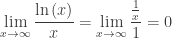So the original area is $\displaystyle \int_{a}^{b}{f\left( x \right)dx}$ and the final area is $L\left( b-a \right)$ . Since these are the same, we can write an equation and solve it for L.

$\displaystyle L\left( b-a \right)=\int_{a}^{b}{f\left( x \right)dx}$

$\displaystyle L=\frac{\int_{a}^{b}{f\left( x \right)dx}}{b-a}$

But that’s the equation for the average value of a function!

What a surprise!

Well, not a surprise for you, the teacher. This might be a good way to sneak up on the average value of a function idea for your students while giving them a good visual idea of the concept.

A Vector’s Derivatives

Posted on January 14, 2015 by Lin McMullin

A question on the AP Calculus Community bulletin board this past Sunday inspired me to write this brief outline of what the derivatives of parametric equations mean and where they come from.

The Position Equation or Position Vector

A parametric equation gives the coordinates of points (x, y) in the plane as functions of a third variable, usually t for time. The resulting graph can be thought of as the locus of a point moving in the plane as a function of time. This is no different than giving the same two functions as a position vector, and both approaches are used. (A position vector has its “tail” at the origin and its “tip” tracing the path as it moves.)

For example, the position of a point on the flange of a railroad wheel rolling on a horizontal track (called a prolate cycloid) is given by the parametric equations

$x\left( t \right)=t-1.5\sin \left( t \right)$

$y\left( t \right)=1-1.5\cos \left( t \right)$ .

Or by the position vector with the same components $\left\langle t-1.5\sin \left( t \right),1-1.5\cos \left( t \right) \right\rangle$ .

Derivatives and the Velocity Vector

The instantaneous rate of change in the y-direction is given by dy/dt, and dx/dt gives the instantaneous rate of change in the x-direction. These are the two components of the velocity vector $\displaystyle \vec{v}\left( t \right)=\left\langle \frac{dx}{dt},\frac{dy}{dt} \right\rangle$ .

In the example, $\displaystyle \vec{v}\left( t \right) =\left\langle 1-1.5\cos \left( t \right),1.5\sin \left( t \right) \right\rangle$ . This is a vector pointing in the direction of motion and whose length, $\displaystyle \sqrt{{{\left( \frac{dx}{dt} \right)}^{2}}+{{\left( \frac{dy}{dt} \right)}^{2}}}$ , is the speed of the moving object.

In the video below the black vector is the position vector and the red vector is the velocity vector. I’ve attached the velocity vector to the tip of the position vector. Notice how the velocitiy’s length as well as its direction changes. The velocity vector pulls the object in the direction it points and there is always tangent to the path. This can be seen when the video pauses at the end and in the two figures at the end of this post.

The slope of the tangent vector is the usual derivative dy/dx. It is found by differentiating dy/dt implicitly with respect to x. Therefore, $\displaystyle \frac{dy}{dx}=\frac{dy}{dt}\cdot \frac{dt}{dx}$ .

There is no need to solve for t in terms of x since dt/dx is the reciprocal of dx/dt, instead of multiplying by dt/dx we can divide by dx/dt: $\displaystyle \frac{dy}{dx}=\frac{dy/dt}{dx/dt}$ .

In the example, $\displaystyle \frac{dy}{dx}=\left( 1.5\sin \left( t \right) \right)\frac{dt}{dx}=\left( 1.5\sin \left( t \right) \right)\left( \frac{1}{1-1.5\cos \left( t \right)} \right)=\frac{1.5\sin \left( t \right)}{1-1.5\cos \left( t \right)}$

Second Derivatives and the Acceleration Vector

The components of the acceleration vector are just the derivatives of the components of the velocity vector

In the example, $\displaystyle \vec{a}\left( t \right)=\left\langle 1.5\sin \left( t \right),1.5\cos \left( t \right) \right\rangle$

The usual second derivative $\displaystyle \frac{{{d}^{2}}y}{d{{x}^{2}}}$ is found by differentiating dy/dx, which is a function of t, implicitly with respect to x:

$\displaystyle \frac{{{d}^{2}}y}{d{{x}^{2}}}=\left( \frac{d}{dt}\left( \frac{dy}{dx} \right) \right)\left( \frac{dt}{dx} \right)=\frac{\frac{d}{dt}\left( dy/dx \right)}{dx/dt}$

In the example,

$\displaystyle \frac{{{d}^{2}}y}{d{{x}^{2}}}=\left( \frac{d}{dt}\left( \frac{1.5\sin \left( t \right)}{1-1.5\cos \left( t \right)} \right) \right)\left( \frac{1}{1-1.5\cos \left( t \right)} \right)$

$\displaystyle =\frac{\left( 1-1.5\cos \left( t \right) \right)\left( 1.5\cos \left( t \right) \right)-\left( 1.5\sin \left( t \right) \right)\left( 1.5\sin \left( t \right) \right)}{{{\left( 1-1.5\cos \left( t \right) \right)}^{2}}}\cdot \frac{1}{\left( 1-1.5\cos \left( t \right) \right)}$

$\displaystyle =\frac{1.5\cos \left( t \right)-{{1.5}^{2}}}{{{\left( 1-1.5\cos \left( t \right) \right)}^{3}}}$

The acceleration vector is the instantaneous rate of change of the velocity vector. You may think of it as pulling the velocity vector in the same way as the velocity vector pulls the moving point (the tip of the position vector). The video below shows the same situation as the first with the acceleration vectors in green attached to the tip of the velocity vector.

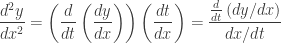
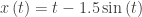
Here are two still figures so you can see the relationships. On the left is the starting position t = 0 with the y-axis removed for clarity. At this point the red velocity vector is $\left\langle -0.5,0 \right\rangle$ indicating that the object will start by moving directly left. The green acceleration vector is $\left\langle 0,1.5 \right\rangle$ pulling the velocity and therefore the object directly up. The second figure shows the vectors later in the first revolution. Note that the velocity vector is in the direction of motion and tangent to the path shown in blue.

Euler’s Method

Posted on January 12, 2015 by Lin McMullin

Differential Equations 3 – Euler’s Method

Since not all differential equation initial values problems (IVP) can be solved, it is often necessary to approximate the solution. There are several ways of doing this. The one that AP students are required to know is Euler’s Method.

The idea behind Euler’s Method is to first write the equation of the line tangent to the solution at the initial condition point. To find the approximate value of the solution near the initial condition, then take short steps from the initial point to the point with the x-value you need.

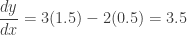
Since you have the initial point and the differential equation will give you the slope, it is easy to write the equation of the tangent line. You then approximate the point on the solution by using the point on this line a short distance (called the step-size or $\Delta x$ ) from the initial point. The first step is exactly the local linear approximation idea.

Next, you write the equation of another line through the approximated point using the differential equation to give you the slope at the approximated point (i.e. not the point on the curve which you do not know). This gives you a second (approximate) point.

Then you repeat the process (called iteration) until you get to the x-value you need.

The equations look like this:

$x_{n}={{x}_{n-1}}+\Delta x$

${{y}_{n}}={{y}_{n-1}}+{f}'({{x}_{n-1}},{{y}_{n-1}})\Delta x$

The first equation says that the x-values increase by the same amount each time. $\Delta x$ may be negative if the required value is at an x-value to the left of the initial point.

The second equation gives the y-value of a point on the line through the previous point where the slope, ${f}'({{x}_{n-1}},{{y}_{n-1}})$ , is found by substituting the coordinates of the previous point into the differential equation. It has the form of the equation of a line.

Example: Let f be the solution of the differential equation $\displaystyle \frac{dy}{dx}=3x-2y$ with the initial point (1, 3). Approximate the value of f(2) using Euler’s method with two steps of equal size.

Solution: At the initial point $\displaystyle \frac{dy}{dx}=3(1)-2(3)=-3$ . Then

${{x}_{1}}=1.5$ and ${{y}_{1}}=3+(3(1)-2(3))(0.5)=1.5$

Now using the point (1.5, 0.5) where $\displaystyle \frac{dy}{dx}=3(1.5)-2(0.5)=3.5$

${{x}_{2}}=2$ and ${{y}_{2}}=0.5+(3.5)(0.5)=2.25$

Therefore, $\left( 2 \right)\approx 2.25$ . The exact value is 2.5545. A better approximation could be found using smaller steps.

Some textbooks and some teachers make tables to organize this procedure. This is fine, but not necessary on the AP exams. Showing the computations as above will earn the credit. It is easy to remember: you are just writing the equation of a line.

There are calculator programs available on-line that will compute successive iterations of Euler’s method and others that will compute and graph the values so you can examine the approximate solution graph. Of course in real situations computers using this or more advanced techniques can produce approximate numerical solutions to initial value problems.

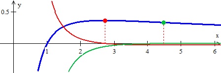
Here is a graphical look at what Euler’s Method does. Consider this easy IVP: $\displaystyle \frac{dy}{dx}={{e}^{x}}$ with the initial condition $y\left( 0 \right)=1$ . The screen is two units wide extending from x = 0 to x = 2. The calculator graph below shows three graphs. The top graph is the particular solution $y={{e}^{x}}$ . (I said it was easy.) The lower graph shows an approximate solution with the rather large step size of $\Delta x=1$ with the two points connected; look closely and you will see the two segments. The middle graph has a step size of $\Delta x=0.25$ . There are 8 segments, but they appear to be a smooth curve approximating the solution. Notice it is closer to the actual solution graph. An even smaller step size would show an even smoother graph closer to the particular solution.

Slope Fields

Posted on January 9, 2015 by Lin McMullin

Differential Equation 2 – Slope Fields

Of course, we always want to see the graph of an equation we are studying. The graph of a differential equation is a slope field. A first derivative expressed as a function of x and y gives the slope of the tangent line to the solution curve that goes through any point in the plane.

Slope fields make use of this by imposing a grid of points evenly spaced across the Cartesian plane. At each point the value of the derivative is calculated and a short segment with that slope is drawn. These segments graphed together form the slope field.

Here is the slope field for the differential equation $\displaystyle \frac{dy}{dx}=-\frac{x}{y}$

A good way to introduce slope fields to your class is to put or project a coordinate system on the board. Give each student one or two points (1, –3), (1, –2), (1, –1), (1, 1), (1, 2), etc. Have them calculate the derivative at their point(s) and then come to the board and draw a short segment through their point(s) with the slope they calculated. The result will be a slope field. (This is, in fact, a common free-response question on the AP exams. Students are given a graph with 9 – 12 points plotted and they are asked to use them to draw a slope field for a given differential equation.)

The big idea with slope fields is to use them to get an idea of what the solutions look like, especially if the differential equation cannot be solved. The solutions are lurking in the slope field. What do they look like in the figure? Circles of course. We solved this differential equation in the last post. The general solution is ${{x}^{2}}+{{y}^{2}}={{C}^{2}}$ . Of course, they are not all that simple.

Since the solution graphs are lurking in the slope field, the next thing to do is to use the slope field to sketch a particular solution. After plotting the initial condition (a point) students should draw a curve through the point that follows the slope field from edge to edge in both directions.

In the previous post (example 2) we found the particular solution of $\displaystyle \frac{dy}{dx}=-\frac{x}{y}$ with the initial condition point (4, –3) to be $y=-\sqrt{25-{{x}^{2}}}$ . This is shown drawn on the slope field in the next graph. The black dot is the point (4, –3). Notice how the solution graph follows the slope field, but does not necessarily hit any of the segments. The solution will touch a segment only if the midpoint of the segment happens to be on the solution – this is not usually the case.

Slope fields are tedious and time-consuming to draw by hand. It’s a job for computers. There are various graphing calculator programs available on the internet. Calculator screens are not the best for seeing slope fields; they are too small, and you should be sure to always be in a square window (or the slopes will not look right).

There are many websites that will draw slope fields and solution curves for you. You can try this one. The figures in this post were done with Winplot (of course, my favorite). The good ones let you draw and animate solution curves over the slope field. (I have not found a good slope field generator app for iPads; if anyone makes apps, consider this a hint.)

Here is a brief example that shows how powerful an animated graph can be. In Winplot, follow the path Window > 2-dim > Equa > differential > dy/dx. Enter the differential equation in the box and adjust the other settings as necessary. Be sure you are in a square window (CTRL+Q).

The example below is from the 2002 BC exam question 5: $dy/dx=2y-4x$ . Notice that this equation is not separable; students were not expected to solve it. They were asked to draw the solution curves through the two points (0, 1) and (0, –1) shown here in blue. These points are marked on the graph (Equa > point > (x,y)). The general solution, found by CAS, is $y=C{{e}^{2x}}+2x+1$ . Enter this (Equa > 1.Explicit) and open the C slider (Anim > individual > C).

In the video below the C values go from –5 to 5. They stop momentarily at the two initial condition points (C = –2 for (0,–1) and C = 0 for (0, 1)). These are what the students were expected to sketch.

The point is to see how the different values of C affect the equation, each giving its own particular solution, and to see the different solution hiding in the slope field.

Winplot may be downloaded here.

A DESMOS program that will draw slope fields is here.

Teaching Calculus

The pleasure lies not in discovering the truth, but in searching for it.

Author Archives: Lin McMullin

Graphing Calculators

February 2015

Yitang Zhang

Good Question 1: 2008 AB 6

Half-full and Half-empty

A Vector’s Derivatives

Euler’s Method

Slope Fields

Share this:

Yitang Zhang

Share this:

Share this:

Share this:

Share this:

Share this:

Share this: