
The goals of the AP Calculus program state that, “Students should be able to communicate mathematics and explain solutions to problems both verbally and in well written sentences.” For obvious reasons the verbal part cannot be tested on the exams; it is expected that you will do that in your class. The exams do require written answers to a number of questions. The number of points riding on written explanations on recent exams is summarized in the table below.
| Year | AB | BC |
| 2007 | 9 | 9 |
| 2008 | 7 | 8 |
| 2009 | 7 | 3 |
| 2010 | 7 | 7 |
| 2011 | 7 | 6 |
| 2012 | 9 | 7 |
| 2013 | 9 | 7 |
| 2014 | 6 | 3 |
The average is between 6 and 8 points each year with some years having 9. That’s the equivalent of a full question. So this is something that should not be overlooked in teaching the course and in preparing for the exams. Start long before calculus; make writing part of the school’s math program.
That a written answer is expected is indicated by phrases such as:
- Justify you answer
- Explain your reasoning
- Why?
- Why not?
- Give a reason for your answer
- Explain the meaning of a definite integral in the context of the problem.
- Explain the meaning of a derivative in the context of the problem.
- Explain why an approximation overestimates or underestimates the actual value
How do you answer such a question? The short answer is to determine which theorem or definition applies and then show that the given situation specifically meets (or fails to meet) the hypotheses of the theorem or definition.
Explanations should be based on what is given in the problem or what the student has computed or derived from the given, and be based on a theorem or definition. Some more specific suggestions:
- To show that a function is continuous show that the limit (or perhaps two one-sided limits) equals the value at the point. (See 2007 AB 6)
- Increasing, decreasing, local extreme values, and concavity are all justified by reference to the function’s derivative. The table below shows what is required for the justifications. The items in the second column must be given (perhaps on a graph of the derivative) or must have been established by the student’s work.
| Conclusion | Establish that |
| y is increasing | y’ > 0 (above the x-axis) |
| y is decreasing | y’ < 0 (below the x-axis) |
| y has a local minimum | y’ changes – to + (crosses x-axis below to above) or  |
| y has a local maximum | y’ changes + to – (crosses x-axis above to below) or  |
| y is concave up | y’ increasing (going up to the right) or  |
| y is concave down | y’ decreasing (going down to the right) or  |
| y has point of inflection | y’ extreme value (high or low points) or  changes sign. changes sign. |
- Local extreme values may be justified by the First Derivative Test, the Second Derivative Test, or the Candidates’ Test. In each case the hypotheses must be shown to be true either in the given or by the student’s work.
- Absolute Extreme Values may be justified by the same three tests (often the Candidates’ Test is the easiest), but here the student must consider the entire domain. This may be done (for a continuous function) by saying specifically that this is the only place where the derivative changes sign in the proper direction. (See the “quiz” below.)
- Speed is increasing on intervals where the velocity and acceleration have the same sign; decreasing where they have different signs. (2013 AB 2 d)
- To use the Mean Value Theorem state that the function is continuous and differentiable on the interval and show the computation of the slope between the endpoints of the interval. (2007 AB 3 b, 2103 AB3/BC3)
- To use the Intermediate Value Theorem state that the function is continuous and show that the values at the endpoints bracket the value in question (2007 AB 3 a)
- For L’Hôpital’s Rule state that the limit of the numerator and denominator are either both zero or both infinite. (2013 BC 5 a)
- The meaning of a derivative should include the value and (1) what it is (the rate of change of …, velocity of …, slope of …), (2) the time it obtains this value, and (3) the units. (2012 AB1/BC1)
- The meaning of a definite integral should include the value and (1) what the integral gives (amount, average value, change of position), (2) the units, and (3) what the limits of integration mean. One way of determining this is to remember the Fundamental Theorem of Calculus
. The integral is the difference between whatever f represents at b and what it represents at a. (2009 AB 2 c, AB 3c, 2013 AB3/BC3 c)
- To show that a theorem applies state and show that all its hypotheses are met. To show that a theorem does not apply show that at least one of the hypotheses is not true (be specific as to which one).
- Overestimates or underestimates usually depend on the concavity between the two points used in the estimates.
A few other things to keep on mind:
- Avoid pronouns. Pronouns need antecedents. “It’s increasing because it is positive on the interval” is not going to earn any points.
- Avoid ambiguous references. Phrases such as “the graph”, “the derivative” , or “the slope” are unclear. When they see “the graph” readers are taught to ask “the graph of what?” Do not make them guess. Instead say “the graph of the derivative”, “the derivative of f”, or “the slope of the derivative.”
- Answer the question. If the question is a yes or no question then say “yes” or “no.” Every year students write great explanations but never say whether they are justifying a “yes” or a “no.”
- Don’t write too much. Usually a sentence or two is enough. If something extra is in the explanation and it is wrong, then the credit is not earned even though the rest of the explanation is great.
As always, look at the scoring standards from past exam and see how the justifications and explanations are worded. These make good templates for common justifications. Keep in mind that there are other correct ways to write the justifications.
QUIZ
Here is a quiz that can help your students learn how to write good explanations.
Let
for
. Find the location of the minimum value of f(x). Justify your answer three different ways (without reference to each other).
The minimum value occurs at x = 2. The three ways to justify this are the First Derivative Test, the Second Derivative Test and the Candidates’ Test. (Don’t tell your students what they are – they should know that.) Then compare and contrast the students’ answers. Let them discuss and criticize each other’s answers.


 There are actually several algorithms for square roots and others for cube roots.
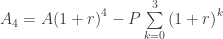
 with the condition A(0) = P. Solving this equation gives
  , but let’s ignore this for now.
 and use (0, P) as the “starting point.”


 instead, you would arrive at the points
 , and
, and  , and
, and  .
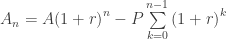
. , the point after t years is
 , the y-value for continuously compounding. This is the solution of the differential equation mentioned above.
 , that is if the derivative is a function of x only, then Euler’s method is the same as a left Riemann sum approximation.
 , and use Euler’s Method with 4 steps starting at (0, 0) and then a left-Riemann sum with 4 terms to approximate
  , (Answer:
  )
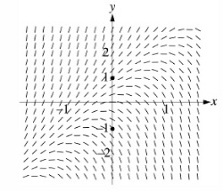
) and its slope field and discussed the questions asked on the exam. Then we saw how to actually solve the equation and found the general solution to be
  .
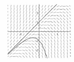
. and realize that e2x is always positive, we can see that solutions with C > 0 lie above the line and those with C < 0 lie below.
 , that is where
  or
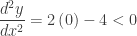
or  . We know they are maximums by the second derivative test:
  when C < 0. All the curves with C < 0 are concave down on their entire domain.
 only those with C < 0 will have maximums.
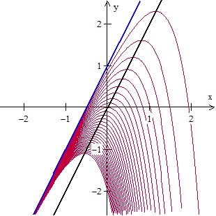

 or
or  . In other words, when the curve lies above the line y= 2x + 1, exactly those with C > 0.
 , and for C < 0,
  .
.


 , ignoring the –4x for the moment. This is easily solved by separating the variables
  , which can be checked by substituting.


 . This may be checked by substituting. Notice that when C = 0 the particular solution is y = 2x + 1, the line through the point (0, 1).

 = the original amount plus the interest on this amount minus the payment, P.
 =
=  , minus the payment, P.


 .
.
 .
. .
.