Good Question 14

Posted on February 23, 2018 by Lin McMullin

Good Question 14 – The Integral Test

I have no criteria for what constitutes a “Good Question” for this series of occasional posts. They are just questions that I found interesting, or that seem more than usually instructive, or that I learn something from. I cannot quote this question (2016 BC 92) since it is on a secure exam. What made it interesting is that to answer it students pretty much needed to know the proof of the Integral Test and the figures that go with it.

I recall only one AP question from many years ago that asked students to “prove” something – usually students are asked to show that a result was true by citing the theorem that applied and showing the hypotheses were met. The directions are often “justify your answer.”

Doing an original proof is not, in my opinion, a fair question and proving some known theorem is just a matter of memorization. For these reasons, students are not asked to prove things on the exams. So, should you prove things in class? Probably, yes.

Here is the usual proof of the integral test. Afterwards I’ll discuss the question from the exam.

The Integral Test

Hypotheses: Let $f\left( x \right)$ be a function that is positive, decreasing, and continuous for $x\ge 1$ ; and let ${{a}_{n}}=f\left( n \right)$ for $x\ge 1$

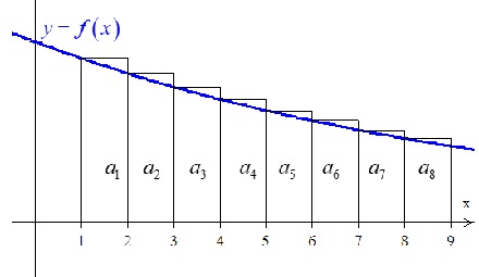
In the first drawing the rectangles have a height of a_n and a width of 1. The area is of each is a_n, and the sum of their areas the series is $\sum\limits_{{n=1}}^{\infty }{{{{a}_{n}}}}$ .

Part 1: Notice that $\sum\limits_{{n=1}}^{\infty }{{{{a}_{n}}}}>\int_{1}^{\infty }{{f\left( x \right)dx}}$ Assume that the improper integral $\int_{1}^{\infty }{{f\left( x \right)dx}}$ diverges.

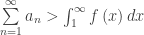
Conclusion 1: If the improper integral $\int_{1}^{\infty }{{f\left( x \right)dx}}$ diverges, then the series $\sum\limits_{{n=1}}^{\infty }{{{{a}_{n}}}}$ diverges.
Conclusion 2: (The contrapositive of conclusion 1) If the series $\sum\limits_{{n=1}}^{\infty }{{{{a}_{n}}}}$ converges, then the improper integral $\int_{1}^{\infty }{{f\left( x \right)dx}}$ converges.

Part 2: In the second drawing below, assume that the improper integral $\int_{1}^{\infty }{{f\left( x \right)dx}}$ converges. The sum of the areas of the rectangles is $\sum\limits_{{n=2}}^{\infty }{{{{a}_{n}}}}$ . (NB: this series starts at n = 2.) Since $\sum\limits_{{n=2}}^{\infty }{{{{a}_{n}}}}$ is less than the convergent improper integral it will also converge. Adding ${{a}_{1}}$ to this gives the original series, $\sum\limits_{{n=1}}^{\infty }{{{{a}_{n}}}}$ ; this series also converges.

Conclusion 3: If the improper integral $\int_{1}^{\infty }{{f\left( x \right)dx}}$ converges, then the series $\sum\limits_{{n=1}}^{\infty }{{{{a}_{n}}}}$ converges.
Conclusion 4: (The contrapositive of conclusion 3) If the series $\sum\limits_{{n=1}}^{\infty }{{{{a}_{n}}}}$ diverges, then the improper integral $\int_{1}^{\infty }{{f\left( x \right)dx}}$ diverges.

Putting the four conclusions together is the Integral Test: If the hypotheses above are met, then the series and the improper integral will both converge, or both diverge.

To answer the multiple-choice question (2106 BC 92) on the exams students were told that the improper integral converges. Therefore, the associated series converges. They then had to determine whether the series or the improper integral has the greater value. Stop here and see if you can figure that out.

Return to the first figure above, only this time assume that the improper integral and the series converge. It is pretty obvious that $\sum\limits_{{n=1}}^{\infty }{{{{a}_{n}}}}>\int_{1}^{\infty }{{f\left( x \right)dx}}$ .

So, even though students were not asked to prove anything, a familiarity with the proof and its figures is necessary to answer the question. That’s why I liked it,

On the other hand, it is kind of an obscure point and I’m not sure it has any practical value.

Polar Equations

Posted on February 20, 2018 by Lin McMullin

Ideally, as with parametric and vector functions, polar curves should be introduced and covered thoroughly in a pre-calculus course. Questions on the BC exams have been concerned with calculus ideas related to polar curves. Students have not been asked to know the names of the various curves (rose, curves, limaçons, etc.). The graphs are usually given in the stem of the problem, but students should know how to graph polar curves on their calculator, and the simplest by hand.

What students should know how to do:

Calculate the coordinates of a point on the graph,
Find the intersection of two graphs (to use as limits of integration).
Find the area enclosed by a graph or graphs: Area = $\displaystyle A=\tfrac{1}{2}\int_{{{\theta }_{1}}}^{{{\theta }_{2}}}{(r(}$ θ $\displaystyle ){{)}^{2}}d$ θ
Use the formulas $x\left( \theta \right)\text{ }=~r\left( \theta \right)\text{cos}\left( \theta \right)~~\text{and}~y\left( \theta \right)\text{ }=~r(\theta )\text{sin}\left( \theta \right)~$ to convert from polar to parametric form,
Calculate $\displaystyle \frac{dy}{d\theta }$ and $\displaystyle \frac{dx}{d\theta }$ (Hint: use the product rule on the equations in the previous bullet).
Discuss the motion of a particle moving on the graph by discussing the meaning of $\displaystyle \frac{dr}{d\theta }$ (motion towards or away from the pole), $\displaystyle \frac{dy}{d\theta }$ (motion in the vertical direction) or $\displaystyle \frac{dx}{d\theta }$ (motion in the horizontal direction).
Find the slope at a point on the graph, $\displaystyle \frac{dy}{dx}=\frac{dy/d\theta }{dx/d\theta }$ .

This topic appears only occasionally on the free-response section of the exam instead of the Parametric/vector motion question. The most recent on the released exams were in 2007, 2013, 2014, and 2017. If the topic is not on the free-response then 1, or maybe 2 questions, probably finding area, can be expected on the multiple-choice section.

Shorter questions on these ideas appear in the multiple-choice sections. As always, look over as many questions of this kind from past exams as you can find.

Here are the few post I have written on polar curves and polar graphing.

Limaçons A discussion of how polar curves are graphed

Back in the summer of 2014 I got interested in some polar equations and wrote a series of post on them which include some gifs showing how they are graphed. They are nothing that will appear on the AP exams. You can use them as enrichment if you like.

Rolling Circles

Roulettes and Calculus

Epitrochoids

Epicycloids

Hypocycloids and Hypotrochoids

Roulettes and Art – 1

Roulettes and Art – 2

What Convergence Test Should I Use? Part 2

Posted on February 16, 2018 by Lin McMullin

In last Friday’s post I really didn’t answer this question. Rather, I tried to show that there is not only one convergence test that must be used on a given series. Nevertheless, the form of a series suggests a test that is likely to work. In this post, I’ll try to give some suggestions as to what test to try first based on the form of the series.

For reference, click here for a table summarizing the common convergence tests.

The goal is for students to be able to decide which test to start with at a glance.

Start with the n^th-term test for divergence. If the limit of the general term as n goes to infinity is not zero, the sequence will diverge. The $\underset{{n\to \infty }}{\mathop{{\lim }}}\,{{a}_{n}}=0$ is a necessary condition for convergence. It is not sufficient; if the limit is zero then the series may converge. Look for a convergence test.

If the series alternates plus and minus signs, it is an alternating series and if it satisfies the other hypotheses use the Alternating Series Test. If the series contains positive and negative signs that do not alternate, or one of the other hypotheses is not met, then a different test must be used.

If the series is geometric then the Geometric Series Test may be used. If the common ratio (the number multiplied by each term to get the next term) is between –1 and 1 the series converges. If the common ratio is greater than or equal to 1, or less than or equal to –1, the series diverges.

The remaining tests are for series with all positive terms. They are tests for absolute convergence. If you series has negative terms then you may ignore the signs and try one of the following tests. If your series is absolutely convergent, then it is convergent. (If not, it may still be convergent.)

If the general term (written with x’s) looks like something that you can integrate, use the Integral Test.

The Direct Comparison Test and the Limit Comparison Test are used if you can find a test to compare them with.

A p-series, $\sum\limits_{{n=1}}^{\infty }{{\frac{1}{{{{n}^{p}}}}}}$ converges if $p>1$ and diverges if $p\le 1$ . A p-series is often a good test to use for comparison in the next two tests. However, any series whose convergence you are sure of may be used.

The Direct Comparison Test is used with fraction expressions. “Extra” factors in the denominator can often be ignored. Some examples

$\displaystyle \sum\limits_{{n=1}}^{\infty }{{\frac{1}{{{{5}^{n}}\sqrt{n}}}}}$ would be a geometric series except for the radical. Compare it with the geometric series $\displaystyle \sum\limits_{{n=1}}^{\infty }{{\frac{1}{{{{5}^{n}}}}}}$
$\displaystyle \sum\limits_{{n=1}}^{\infty }{{\frac{{{{n}^{2}}}}{{{{n}^{4}}+2n+1}}}}$ can be compared with the p-series $\displaystyle \sum\limits_{{n=1}}^{\infty }{{\frac{1}{{{{n}^{2}}}}}}$ . The hint here is that ignoring the lower power terms in the denominator and reducing we see that the original series looks like $\displaystyle \sum\limits_{{n=1}}^{\infty }{{\frac{1}{{{{n}^{2}}}}}}$ . Both series converge. But be careful $\displaystyle \sum\limits_{{n=1}}^{\infty }{{\frac{{{{n}^{2}}}}{{{{n}^{4}}-2n-1}}}}$ while similar, has terms greater than the terms of $\displaystyle \sum\limits_{{n=1}}^{\infty }{{\frac{1}{{{{n}^{2}}}}}}$ .)
The terms of the series $\displaystyle \sum\limits_{{n=1}}^{\infty }{{\frac{1}{{{{{\left( {{{n}^{2}}+2} \right)}}^{{1/3}}}}}}}$ are larger than the harmonic series $\displaystyle \sum\limits_{{n=1}}^{\infty }{{\frac{1}{n}}}$ a divergent p-series, so this series diverges.

The Limit Comparison Test may be used with the same kinds of series that are messy to use with direct comparison.

Returning to $\displaystyle \sum\limits_{{n=1}}^{\infty }{{\frac{{{{n}^{2}}}}{{{{n}^{4}}+2n+1}}}}$ , try the limit comparison test with $\displaystyle \sum\limits_{{n=1}}^{\infty }{{\frac{1}{{{{n}^{2}}}}}}$ . The limit is 1, so both series converge.
$\displaystyle \sum\limits_{{n=1}}^{\infty }{{\frac{1}{{\sqrt{{{{n}^{2}}+3}}}}}}$ Series with radicals also are candidates for the limit comparison test. Since the general terms is approximately $\displaystyle {\frac{1}{n}}$ Compare this with $\displaystyle \sum\limits_{{n=1}}^{\infty }{{\frac{1}{n}}}$ . Both series diverge.

More complicated series, perhaps with exponential factors and/or factorials can be examined with the Ratio Test.

$\displaystyle \sum\limits_{{n=1}}^{\infty }{{\frac{{{{3}^{n}}}}{{n!}}}}$ or $\displaystyle \sum\limits_{{n=1}}^{\infty }{{\frac{{{{n}^{3}}}}{{{{5}^{n}}}}}}$ are candidates for the Ratio Test. Both Converge.
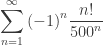
$\displaystyle \sum\limits_{{n=1}}^{\infty }{{{{{\left( {-1} \right)}}^{n}}\frac{{n!}}{{{{{500}}^{n}}}}}}$ appears to be a candidate for the alternating series test. However, for large values of n > 530 the terms increase in absolute vale, so the alternating series test cannot be applied. The ratio test works here, but since the terms do not approach 0 as n increases, the n^th-term test for divergence also works. This series diverges.

Practice, Practice, Practice

The AP Calculus BC exams rarely, if ever, specify which test to use. Often these are multiple-choice questions. If students can see whether the series converges or diverges, that is enough. But here again the key is practice, practice, practice.

As you teach the various tests, pause to look at the form of the series in the exercises for each test that your book provides. Most books also have mixed sets of exercises where tests other than the one in that section are needed. One of the things you can do is assign these entire sets with the directions that students should determine what test they would try, and, for their comparison tests, to which series they would compare it. Discuss their opinions especially if there is more than one suggested or suggest others. Work only those those students are confused about or those for which they have divergent opinions; try to converge on a good test for each.

Revised July 18, 2021, January 29, 2023

Parametric and Vector Equations

Posted on February 13, 2018 by Lin McMullin

In the plane, the position of a moving object as a function of time, t, can be specified by a pair of parametric equations $x=x\left( t \right)\text{ and }y=y\left( t \right)$ or the equivalent vector $\left\langle x\left( t \right),y\left( t \right) \right\rangle$ . The path is the curve traced by the parametric equations or the tips of the position vector. .

The velocity of the movement in the x- and y-direction is given by the vector $\left\langle {x}'\left( t \right),{y}'\left( t \right) \right\rangle$ . The vector sum of the components gives the direction of motion. Attached to the tip of the position vector this vector is tangent to the path pointing in the direction of motion.

The length of this vector is the speed of the moving object. $\text{Speed }=\sqrt{{{\left( {x}'\left( t \right) \right)}^{2}}+{{\left( {y}'\left( t \right) \right)}^{2}}}$ . (Notice that this is the same as the speed of a particle moving on the number line with one less parameter: On the number line $\text{Speed}=\left| v \right|=\sqrt{{{\left( {x}'\left( t \right) \right)}^{2}}}$ .)

The acceleration is given by the vector $\left\langle {{x}'}'\left( t \right),{{y}'}'\left( t \right) \right\rangle$ .

What students should know how to do:

Vectors may be written using parentheses, ( ), or pointed brackets, $\left\langle {} \right\rangle$ , or even $\vec{i},\vec{j}$ form. The pointed brackets seem to be the most popular right now, but all common notations are allowed and will be recognized by readers.
Find the speed at time t: $\text{Speed }=\sqrt{{{\left( {x}'\left( t \right) \right)}^{2}}+{{\left( {y}'\left( t \right) \right)}^{2}}}$
Use the definite integral for arc length to find the distance traveled $\displaystyle \int_{a}^{b}{\sqrt{{{\left( {x}'\left( t \right) \right)}^{2}}+{{\left( {y}'\left( t \right) \right)}^{2}}}}dt$ . Notice that this is the integral of the speed (rate times time = distance).
The slope of the path is $\displaystyle \frac{dy}{dx}=\frac{{y}'\left( t \right)}{{x}'\left( t \right)}$ . See this post for more on finding the first and second derivatives with respect to x.
Determine when the particle is moving left or right,
Determine when the particle is moving up or down,
Find the extreme position (farthest left, right, up, down, or distance from the origin).
Given the position find the velocity by differentiating; given the velocity find the acceleration by differentiating.
Given the acceleration and the velocity at some point find the velocity by integrating; given the velocity and the position at some point find the position by integrating. These are just initial value differential equation problems (IVP).
Dot product and cross product are not tested on the BC exam, nor are other aspects.

Here are two past post on this topic:

Implicit Differentiation of Parametric Equation

A Vector’s Derivatives

Which Convergence Test Should I Use? Part 1

Posted on February 9, 2018 by Lin McMullin

One common question from students first learning about series is how to know which convergence test to use with a given series. The first answer is: practice, practice, practice. The second answer is that there is often more than one convergence test that can be used with a given series.

I will illustrate this point with a look at one series and the several tests that may be used to show it converges. This will serve as a review of some of the tests and how to use them. For a list of convergence tests that are required for the AP Calculus BC exam click here.

To be able to use these tests the students must know the hypotheses of each test and check that they are met for the series in question. On multiple-choice questions students do not need to how their work, but on free-response questions (such as checking the endpoints of the interval of convergence of a Taylor series) they should state them and say that the series meets them.

For our example we will look at the series $\displaystyle 1-\frac{1}{3}+\frac{1}{9}-\frac{1}{{27}}+\frac{1}{{81}}-+\ldots =\sum\limits_{{n=1}}^{\infty }{{{{{\left( {-\frac{1}{3}} \right)}}^{{n-1}}}}}$

Spoiler: Except for the first two tests to be considered, the other tests are far more work than is necessary for this series. The point is to show that several tests may be used for a given series, and to practice the other tests.

The Geometric Series Test is the obvious test to use here, since this is a geometric series. The common ratio is (–1/3) and since this is between –1 and 1 the series will converge.

The Alternating Series Test (the Leibniz Test) may be used as well. The series alternates signs, is decreasing in absolute value, and the limit of the n^th term as n approaches infinity is 0, therefore the series converges.

The Ratio Test is used extensively with power series to find the radius of convergence, but it may be used to determine convergence as well. To use the test, we find

$\displaystyle \underset{{n\to \infty }}{\mathop{{\lim }}}\,\frac{{\left| {{{{\left( {-\frac{1}{3}} \right)}}^{{n+1}}}} \right|}}{{\left| {{{{\left( {-\frac{1}{3}} \right)}}^{n}}} \right|}}=\frac{1}{3}$ Since the limit is less than 1, we conclude the series converges.

Absolute Convergence

A series, $\sum\limits_{{n=1}}^{\infty }{{{{a}_{n}}}}$ , is absolutely convergent if, and only if, the series $\sum\limits_{{n=1}}^{\infty }{{\left| {{{a}_{n}}} \right|}}$ converges. In other words, if you make all the terms positive, and that series converges, then the original series also converges. If a series is absolutely convergent, then it is convergent. (A series that converges but is not absolutely convergent is said to be conditionally convergent.)

The advantage of going for absolute convergence is that we do not have to deal with the negative terms; this allows us to use other tests.

Applied to our example, if the series $\sum\limits_{{n=1}}^{\infty }{{{{{\left( {\frac{1}{3}} \right)}}^{{n-1}}}}}$ converges, then our series $\sum\limits_{{n=1}}^{\infty }{{{{{\left( {-\frac{1}{3}} \right)}}^{{n-1}}}}}$ will converge absolutely and converge.

The Geometric Series Test can be used again as above.

The Integral Test says if the improper integral $\displaystyle {{\int_{1}^{\infty }{{\left( {\frac{1}{3}} \right)}}}^{x}}dx$ converges, then our original series will converge absolutely.

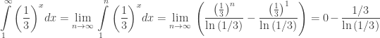
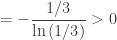
$\displaystyle \int\limits_{1}^{\infty }{{{{{\left( {\frac{1}{3}} \right)}}^{x}}}}dx=\underset{{n\to \infty }}{\mathop{{\lim }}}\,\int\limits_{1}^{n}{{{{{\left( {\frac{1}{3}} \right)}}^{x}}}}dx=\underset{{n\to \infty }}{\mathop{{\lim }}}\,\left( {\frac{{{{{\left( {\frac{1}{3}} \right)}}^{n}}}}{{\ln \left( {1/3} \right)}}-\frac{{{{{\left( {\frac{1}{3}} \right)}}^{1}}}}{{\ln \left( {1/3} \right)}}} \right)=0-\frac{{1/3}}{{\ln \left( {1/3} \right)}}$

$\displaystyle =-\frac{{1/3}}{{\ln \left( {1/3} \right)}}>0$ since ln(1/3) < 0.

The limit is finite, so our series converges absolutely, and therefore converges.

The Direct Comparison Test may also be used. We need to find a positive convergent series whose terms are term-by-term greater than the terms of our series. The geometric series $\sum\limits_{{n=1}}^{\infty }{{{{{\left( {\frac{1}{2}} \right)}}^{{n-1}}}}}$ meets these two requirements. Therefore, the original series converges absolutely and converges.

The Limit Comparison Test is another possibility. Here we need a positive series that converges; we can use $\sum\limits_{{n=1}}^{\infty }{{{{{\left( {\frac{1}{2}} \right)}}^{{n-1}}}}}$ again. We look at

$\displaystyle \underset{{n\to \infty }}{\mathop{{\lim }}}\,\frac{{{{{\left( {1/3} \right)}}^{n}}}}{{{{{\left( {1/2} \right)}}^{n}}}}=\underset{{n\to \infty }}{\mathop{{\lim }}}\,{{\left( {\frac{2}{3}} \right)}^{n}}=0$ and since the series in the denominator converges, our series converges absolutely.

So, for this example all the convergences that may be tested on the AP Calculus BC exam may be used with the single exception of the p-series Test which cannot be used with this series.

Teaching suggestions

While the convergence of the series used here can be done all these ways, other series lend themselves to only one. Stress the form of the series that works with each test. For example, the Limit Comparison Test is most often used for rational expressions with the numerator of lower degree than the denominator and for expressions involving radicals of polynomials. The comparison is made with a p-series of whatever degree will make the numerator and denominator the same degree allowing the limit to be found.
Most textbooks, after explaining each test and giving exercises on them, include a series of mixed exercises that require all the test covered up to that point. A good way to use this set is to assign students to state which test they would try first on each series. Discuss the opinions of the class and work any questions that students are unsure of or on which several ways are suggested.
Give your students the series above, or a similar one, and have them prove its convergence using each of the convergence tests as was done above.
Divide your class into groups and assign each group the series and one of the convergence tests. Ask them to use the test to prove convergence and then discuss the results as a group.

Of course, I didn’t really answer the question, did I? Check What Convergence Test Should I use Part 2

Updated February 23, 2013

More on Power Series

Posted on February 6, 2018 by Lin McMullin

Continuing with post on sequences and series

New Series from Old 1 Rewriting using substitution

New Series from Old 2 Finding series by differentiating and integrating

New Series from Old 3 Rewriting rational expressions as geometric series

Geometric Series – Far Out A look at doing a question the right way and the “wrong” way?

Error Bounds The Alternating Series Error Bound and the Lagrange Error Bound

The Lagrange Highway An example explaining error bounds

Synthetic Summer Fun Using synthetic division, the Remainder Theorem, the Factor Theorem and finding the terms of a Taylor Series (Probably more than you want to know, but possibly an enrichment idea.)

Math vs. the “Real World”

Posted on February 2, 2018 by Lin McMullin

There is a difference between mathematics and the “real world”: In the real world you are allowed to do whatever you want, as long as there is no law against doing it; in mathematics, you cannot do something unless there is a law that says you may.

A question that comes up often on the AP Calculus Community bulletin board concerns the divergence of the improper integral $\displaystyle \int_{{-1}}^{1}{{\frac{1}{x}dx}}$ .

There are several mistakes students make when computing this integral.

First, they may not realize this is an improper integral and compute incorrectly:

$\displaystyle \int_{{-1}}^{1}{{\frac{1}{x}dx}}=\ln \left| 1 \right|-\ln \left| {-1} \right|=0-0=0$

Since the laws concerning improper integrals do not allow this, you may not do it.

Or, they might think that it does converge to zero by the symmetry of the graph. There is no law (theorem) that permits calculating limits based on the appearance of a graph.

Finally, and most often, they may start out following the rules but go astray. The law says you must find deal with the discontinuity at x = 0 by using one-sided limits:

$\displaystyle \int_{{-1}}^{1}{{\frac{1}{x}dx}}=\underset{{a\to 0-}}{\mathop{{\lim }}}\,\int_{{-1}}^{a}{{\frac{1}{x}dx}}+\underset{{b\to 0+}}{\mathop{{\lim }}}\,\int_{b}^{1}{{\frac{1}{x}dx}}$

$=\underset{{a\to 0-}}{\mathop{{\lim }}}\,\left( {\ln \left| a \right|-\ln \left| 1 \right|} \right)+\underset{{b\to 0+}}{\mathop{{\lim }}}\,\left( {\ln \left| 1 \right|-\ln \left| b \right|} \right)$

$=\left( {-\infty -0} \right)+\left( {0-(-\infty )} \right)=\infty -(\infty )=0$

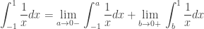
The mistake is subtler here. It is correct to say that $=\underset{{a\to 0-}}{\mathop{{\lim }}}\,\ln \left| a \right|=-\infty$ , but what that really means is that the limit does not exist (DNE). Then in the last line above you cannot say

(does not exist) – (does not exist) = 0.

You cannot subtract something that does not exist from something else that does not exist. As soon as you see that one of the limits does not exist, the entire limit does not exist. (That’s the law.) There is no algebra/calculus theorem that permits the addition of two divergent integrals, therefore, it is not correct to add them.

Students need help in understanding this. Here are three ways to think about it.

Infinity is not a number. When you say the integrals equal infinity and negative infinity, you must stop. Just because it looks like something minus the same thing is zero, you cannot do this, because you’re not working with numbers. In fact, the integrals do not exist, so you cannot add them – there’s nothing to add.
“Infinity” is a short, and correct, way of expressing the limits as you approach zero for this function from the right or left. But, you must remember that infinity is a shorthand for DNE, not for some really large number and its opposite.
Infinity minus infinity ( $\infty -\infty$ ) is an indeterminate form. Some indeterminate forms of this type converge, if you can find some additional algebra/calculus to do on them (such as L’Hospital’s Rule in some cases). For this example, such algebra/calculus does not exist (no pun intended)

So, in conclusion $\displaystyle \int_{{-1}}^{1}{{\frac{1}{x}dx}}$ does not converge!

This question was discussed recently on the AP Calculus bulletin board. The two items below were included and may help your students understand what’s going on with infinity. The are by Stu Schwartz.

Thank You Stu!

Teaching Calculus

The pleasure lies not in discovering the truth, but in searching for it.

Monthly Archives: February 2018

Good Question 14

Polar Equations

What Convergence Test Should I Use? Part 2

Parametric and Vector Equations

Which Convergence Test Should I Use? Part 1

More on Power Series

Math vs. the “Real World”

Share this:

Share this:

Share this:

Share this:

Share this:

Share this:

Share this: