Visualizing Solid Figures 5

Posted on November 25, 2014 by Lin McMullin

To end this series of posts on visualizing solid figures, we will look at a problem that relates to how volumes of solid figures are formed. It has 5 parts which will be presented first. Then the solution will be given.

Consider the region in the first quadrant bounded by the graphs of the parabola $y={{x}^{2}}$ and the line $y=9$ both for $0\le x\le 3$ .

This region is revolved around the y-axis to form a solid figure.

Use the disk/washer method to find the volume of this figure.
Use the method of cylindrical shells to find the volume of this figure.
Use the disk/washer method to find a number j , such that when x = j the volume of the figure is one-half that of the original figure.
Use the method of cylindrical shells to find a number k , such that when x = k the volume of the figure is one-half that of the original figure.
The answers to parts a) and b) should be the same, but the answers to parts c) and d) are different. Explain why they are different.

Solutions:

1. The volume by the disk/washer method is

$\displaystyle V=\int_{0}^{9}{\pi {{x}^{2}}dy}=\int_{0}^{9}{\pi ydy}=\frac{81}{2}\pi \approx 127.235$

2. The volume by the method of cylindrical shells is

$\displaystyle \int_{0}^{3}{2\pi x\left( 9-y \right)dx}=\int_{0}^{3}{2\pi x\left( 9-{{x}^{2}} \right)dx}=\frac{81}{2}\pi \approx 127.235$

3. The value is be found by solving the equation for j:

$\displaystyle \int_{0}^{{{j}^{2}}}{\pi y\,dy}=\frac{81}{4}\pi$ , so $j\approx 2.52269$

4. The value is be found by solving the equation for k:

$\displaystyle \int_{0}^{k}{2\pi x\left( 9-{{x}^{2}} \right)dx}=\frac{81}{4}\pi$ and $k\approx 1.62359$

5. The reason the values are not the same is this. Think of the revolved parabola as a bowl. If you pour water into the bowl until it is half full, the bowl looks like the figure below. The water is pooled in the bottom of the bowl as you would expect. This is what happens when using the disk/washer method. The washers stack up starting in the bottom of the bowl until it is half full.

On the other hand, the method of cylindrical shells sort of wraps the water in layers (the shells) around the y-axis. Picture the water being sprayed on the y-axes and frozen there. Each new layer (shell) increases the amount and you end up half of the total volume arranged as a cylinder with a rounded (paraboloid shaped) bottom as shown in the figure below. Both bowls contain the same amount of water, arranged differently.

Visualizing Solid Figures 4

Posted on November 22, 2014 by Lin McMullin

Volume by the method of “Cylindrical Shells”

Today I will show you how to visualize the cylindrical shells used in computing the volume using Winplot.

Winplot is a free program. Click here for Winplot and here for Winplot for Macs.

For the example I will use the same situation as in the last post. This was an AP question from 2006 AB1 / BC 1. In part (c) students were asked to find the volume of the solid figure formed when the region between the graphs of y = ln(x) and y = x – 2 is revolved around the y-axis. This can be done by the washer method, but some students use the method of cylindrical shells. We found that the graphs intersect at x = 0.15859 and x = 3.14619.

Begin as before by graphing the two functions and the vertical segment joining them.

In Winplot open a 2D window, click on Equa > 1. Explicit and enter the first equation. Click the “lock interval” box and enter 0.159 for the “low x,” and 3.146 for the “high x,” choose a color and click “ok.”
Repeat this for the second equation.
Then return to Equa > Segment > (x,y) and enter the endpoints of the vertical segment joining the graphs: x1 = B, y1 = ln(B), x2 = B, and y2 = B – 2. Choose a color and click “ok.”
Click Anim > individual > B to open a slider box for B. Type 0.159 and click “set L” and then type 3.146 and click “set R.” Use this slider to move the thin Riemann sum rectangle across the region.

Next draw the 3D graphs:

Click One > Revolve Surface. The equations will appear in the drop-down box at the top of the window. Graphs are revolved one at a time. For the first graph click the “y-axis” button to put the correct values for a, b, and c in the boxes. In the “arc start” box type 0.159 and in the “arc stop” box type 3.146, the ends of the interval. In the “angle stop” box type 2pi@S. (S for surface.) See the figure below. Click “see surface.”

Repeat this by selecting the second function from the drop-down box. Leave all the values the same and click enter. The two surfaces will be graphed in the same color as the corresponding functions in the 2D set up.
Repeat this for the segment, but change the 2p@S in “arc stop” box to 2p@R. (R for Riemann rectangle.) Click “see surface.”
You will need to make one adjustment at this point. In the 3D Inventory list choose the segment and click “edit.” In the box change “low t” to 0 and the “high t” to 1. See the next figure.

In the 3D window, click Anim > Individual and open slider boxes for B, R, and S.
In the B box enter 0.159 and click “set L” and enter 3.146 and click “set R.” These are the endpoints.
In the S box make “set L” = -2pi. “Set R” should already be 2pi. Then type 0 and Enter.
The R box should open with “set L” = 0 and “Set R” = 2pi. no changes are necessary.

Move first the B slider, then the R slider, then the B slider again and finally the S slider to explore the situation.
Type Ctrl+A to show the axes. Use the 4 arrow keys to move the figure around, and the page up and page down keys to zoom in and out.

That should do it.

In the video above you will see

The Riemann rectangle moving in the plane using the B slider.
The Riemann rectangle rotated around the y-axis using the R slider.
The shell moving through the curves using the B slider again.
The two curves rotated part way using the S slider.
The shell moving through the solid using the B slider.

The next and last post in this series will be a question to see if you understand how the washer method and the cylindrical shell method work in a real situation.

Update:One of my favorite post is Difficult Problems and Why We Like Them from June 10, 2013. In it I mention a sculpture called Kryptos located at CIA headquarters in Langley, Virginia. The sculpture contains four enciphered messages. Only three of these have been deciphered since the sculpture was erected in 1990. The sculptor has offered a second clue to the fourth message. I’ve added links story and clues in the original post; see if you can decipher the fourth part.

Visualizing Solid Figures 3

Posted on November 19, 2014 by Lin McMullin

Volume by “Washers”

Today I will show you how to visualize not just the solid figures but the disks and washers used in computing the volume using Winplot. The next post will show how to draw shells.

Winplot is a free program. Click here for Winplot and here for Winplot for Macs.

For the example we’ll use the situations from the 2006 AP calculus exams question AB1 / BC 1. The students were given the region between the graphs of y = ln(x) and y = x -2. In the first part they were asked to find the area of the region. To do that they first had to determine, using their calculator, where the curves intersect. The x-coordinates of the intersections are x = 0.15859 and x = 3.14619.

In part (b) they were asked to find the volume of the solid formed when the region was rotated around the horizontal line y = -3 . The volume is found by using the disk/washer method. Here is how to show the washers using Winplot. This gets a little complicated so I will mark each step with a bullet

Starting in the 2D window, graph the two functions as shown in the previous post.. When entering the equations click the “lock interval” box and enter 0.159 for “low x” and 3.146 for “high x.”
Next we will enter a Riemann sum rectangle which we will be able to move, and, once rotated, will appear as the washer. Go to Equa > Segment > (x,y) and in the box enter the endpoints of the vertical segment between the two graphs in terms of B: x1 = B, y1 = ln(B), x2 = B, and y2 = B – 2. Click “ok.”
Go to the Anim button, choose “B” (Anim > Individual > B).
Enter the left value 0.15859 and click “set L”, and enter 3.14619 and click “set R.” (Remember how to do this, as we will do it again.)
You may now move the “Riemann rectangle” (which, of course, is very thin, approaching 0) across the region.

Next we will produce the 3D images.

As we did in the last post click on One > Revolve surface… Enter the values shown below. (The “arc start” and “arc stop” value are the x-values of the intersection points. Attach an “@S” to the “angle stop” as shown.)

Click “see surface.”
In the 3D window that appears click Anim > S and you will be able to revolve the curve. Make the “set L” value -2pi by typing the value in the box and clicking “set L,” leave “set R” at 2pi. Adjust the value to 0 by typing 0 and “enter.”
Adjust the viewing widow with the 4 arrow keys and the Page Up and Page down keys. Add the axes with Ctrl+A.
Return to the “surface of revolution” window and choose the second function from the drop-down box at the top. not change anything else. Click “see surface” and the second curve will be added to the graph.

Next we graph the “washer:”

In the surface of revolution box, select the segment in the drop-down box at the top change the “angle stop” to 2pi@R. Click “ok.”
Then in the 3D Inventory window for this file select the segment and click “edit.”
Change the “low t” value to 0 and the “high t” value to 1. Change the “u hi” to 2pi@R. Click “ok.” The window should look like the one below.

Finally, in the 3D window:

To show the line y = –3, in the 3D window go to Equa > 2. Parametric and enter the values shown in the box below and click “ok.” A short segment at y = -3 will appear in the 3D window.
In the 3D window go to Anim > Individual and open a slider for “B” and for “R.”
For the “B” slider make “set L” = 0.15859 and the “set R” to 3.14619 (the intersection values).
For the “R” slide make “set L” to 0 and “set R” to 2pi.
Adjust the R and S sliders to 0 and the B slider to its minimum value.
Save everything just to be safe. The extension will be “.wp3.” Later you can open this file from the 3D window, but it will no longer be in touch with the 2D window even if you save that.

That should do it.

Move first the B slider, then the R slider, then the B slider again and finally the S slider to explore the situation.

In the video at the top you will see this example with these things happening in order.

The Riemann rectangle moving in the plane using the B slider
The Riemann rectangle rotated into a washer using the R slider.
The washer moving through the curves using the B slider again.
The two curves rotated part way using the S slider
The washer moving through the solid using the B slider.
The solid rotated with the 4 arrow keys.

The next post will show how to do a similar animation for the cylindrical shell method.

Visualizing Solid Figures 2

Posted on November 16, 2014 by Lin McMullin

You have probably caught on by now that Winplot is my favorite computer graphing program. In addition to being great at drawing quick graphs, it is able to produce and rotate 3D images of, among other things, solids of rotation, and solids with regular cross-sections. In this post I will discuss how to do solids of regular cross-section and solids of rotation. In my next posts I’ll show you how to see the disks, washers, and shells.

Winplot is a free program. Click here for Winplot for PC and here for Winplot for Macs. (May 11, 2017 Note: Winplot is no longer available from its original home. The link for PCs above connect to another site where the program can be downloaded. For Macs use the PC link, but use the Winplot for Macs link for instructions and another program you will need.You can also Google Winplot and find other sites that have the program as well as many, many instructional videos.)

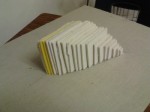
Solids with regular cross-sections

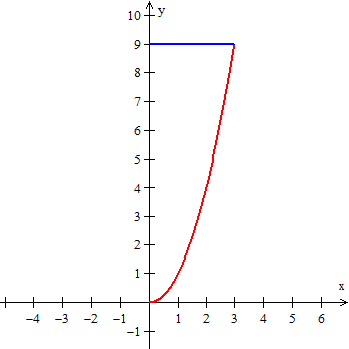
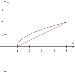
Consider the region bound by the graphs of $f\left( x \right)=\sqrt{x-1}$ and $g\left( x \right)=\tfrac{1}{2}\left( x-1 \right)$ from x = 1 to x = 5.

Begin by opening a Winplot 2D graphing window, graphing the curves, and adjusting the window to a good scale. Use the box where the equations are entered (Equa > 1.Explicit) check “lock interval,” and enter the “low x” and “high x” values (1 and 5 respectively) to stop the graphs where they intersect. Click “ok” to see the graphs.

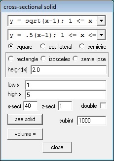
On the navigation bar, click on “Two” and then “Sections.” You should see a window like this:

The top two drop-down boxes at the top allow you to choose which curves to work with, and since we have only two they should already be selected. Then click on the cross-section shape you want – square, equilateral triangle, or semicircle. The box below that allows other shapes where the height may be set (the height(x) may be a number or a function of x). Set the “low x” and “high x” to the left and right sides of the region. Then click “see solid” and you will see the solid in a new window.

Click on the new 3D window and then type Ctrl+A to show the axes. Rotate the image by using the 4 arrow keys, and zoom in and out with the Page Up and Page Down keys.

Now let’s get fancy. Close the 3D window and return to the cross-section box shown above. Change the “high x” to 5@B (you may use any almost letter except x, y, or z). Then click “see solid.” Next, in the 3D Window click Anim > Individual > B. This will give you a slider. Slide the slider from 1 to 5 and you will see the solid grow and see the square cross-sections. (The video uses the “autocyc” button – use S to slow the animation, F to speed it up and Q to quit.)

Use File > Save As… to save the image. It will save with the extension .wp3 and you will lose the original 2D graphs. The animation buttons will still work when you open it again.

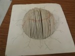
Solids of Revolution.

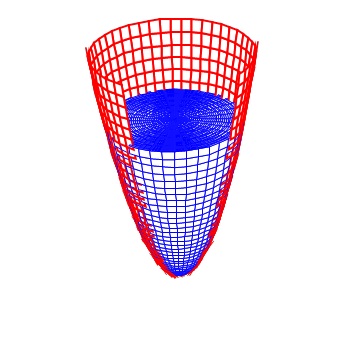
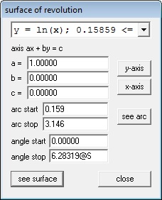
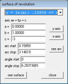
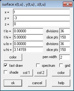
Solids of rotation are done in a similar way. We will revolve the same curves around the horizontal line y = –1. Enter the curves as above and click on One > Revolve Surface. Curves are revolved one at a time, so choose the first curve from the drop-down box. Choose the axis the figure is to be rotated around by entering the values for a, b, and c in ax + by = c, or clicking on one of the axis buttons. For the “arc start” and “arc stop” values use the left and right ends of the region. The “angle start” and “angle stop” values are the default, 0 and 2pi (entered as “2pi”). Again we have made this last value 2pi@A so that we can animate the graph.

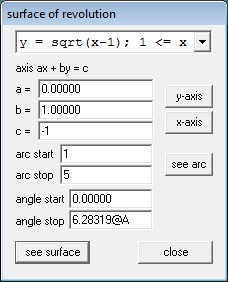
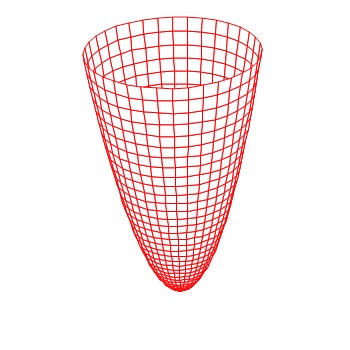
Click “see surface” to see the revolved surface. As before, use the 4 arrow keys and the Page Up and Page Down keys to adjust the image, and Ctrl+A to show the axes.

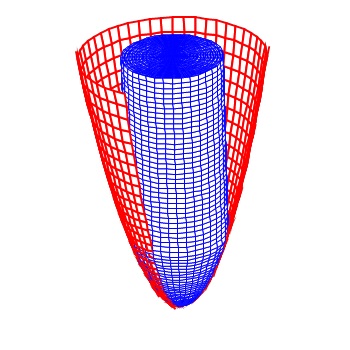
Surfaces are revolved one at a time so return to the “surface of revolution” window and use the drop-down box to choose the next curve. Leave all the other values the same. Clicking “see surface” will graph the second curve with the first and show the solid figure. Note that the surfaces are graphed in the same color as the original 2D graphs.

Use the slider or autorev or autocyc buttons to watch the curves revolve. (Remember to type “F” to speed up the motion. “S” to slow it down, and “Q” to quit.)

The next posts will show how to see the disks, washers, and shells, and animate them along with the surfaces.

Visualizing Solid Figures 1

Posted on November 13, 2014 by Lin McMullin

The shape of various solids of rotation and solids with regular cross-sections of which beginning calculus students are required to find the volume are often difficult to visualize. This post and the next two will discuss some of the ways you can help your students become familiar with these shapes. Teachers often use these as projects for students to get some hands-on familiarity with the figures. In fact, it is one of the few places where a useful project can be assigned.

Actually, rotate a region:

Begin by drawing the region to be revolved (from the curve to the line of rotation) on paper and cut it out. Tape the region along the line to a pencil, pen, or dowel. Roll the dowel back and forth between your hands or, as shown in the video below, with a small electric drill or screwdriver. You can get a rough idea of the shape.

Go to a wedding:

Decorations for weddings and other festive events are made from paper and fold flat. When opened you get a solid of rotation.

Measure a volume:

Take a solid fruit (like a banana), or a vegetable (like a cucumber, or carrot) and find its volume by cutting it into “coin” shaped pieces. Multiply the thickness by the area of the circular ends of each piece and then add them to find the volume.

For more of a challenge use a loaf of sliced bread (here you will need a way to calculate the area of the non-circular ends – inscribed rectangles perhaps). You could also approximate the volume of a tree trunk by measuring the circumference at regular distances along the trunk.

Build a model:

This method can be used for solids or rotation and is especially good for solids with regular cross-sections. It is also a good project for a student or group of students.

Carefully graph the region using a somewhat larger than normal scale.
Draw lines at 1/8 to ¼ inch intervals across the region perpendicular to the appropriate axis.
Carefully measure or calculate the length of each of these lines. Use this for the appropriate dimension for the question. For example, this may be the side of the square cross-section, or the diameter of a semi-circular section.
Use the dimension to draw a series of squares, semi-circles, or whatever from cardboard, plywood, or foam board.
Cut these out and assemble them on the original region you graphed to approximate the solid figure. Tape or glue them in place.
Extra: Calculate the area of each piece and multiply it by the thickness (or the distance between pieces) and see how closely this comes to the calculated volume.

: Square cross-sections from scrap wood.

: Square cross-sections on a circular base made from scrap plywood.

: Trapezoidal sections on parabolic base made from 5.25 inch floppy disks.

: Square cross-sections on base between a parabola and a line made with foam board.

: Semi-circular cross-sections on a circular base made from foam board.

These pictures are of models made by students of Mrs. Dixie Ross at Pflugerville (Texas) High School. Students received more points if they recycled materials.Thank you Dixie!

November

Posted on November 1, 2014 by Lin McMullin

November – deep into derivatives. This month’s featured posts from past Novembers are below. “Speed,” which discusses various ways to approach this topic, seems to be one of the most popular with close to 2600 hits since it was first posted in 2012. This is followed by “Open cor Closed” which discusses a question that almost always comes up at workshop and online: should the interval where a function is increasing or decreasing by open or closed. The next two most popular are “Motion Problems” one of the several posts on inverses.

When I began this blog I was posting about three times per week. I have the whole of first-year calculus to write about. I hope I’ve hit the main points. If there is anything you would like me to add or expand on, or any topic or problem you think others might be interested in please let me know; I can use some ideas.

I did get a request this week to update my Guide to AP Calculus (AB & BC) Free-response Questions. (I meant to do this, but totally forgot about it.) This guide gives suggestions on what is asked on the various common free-response questions. I’ve expanded this in my posts on reviewing for the exam (check the “Thru the Year” tab under January and February). The Guide also list the question number and individual notes on individual questions from 1998 through 2014. The Guide is on the Resource page or you can click the link at the beginning of this paragraph.

Graphing, Inverses, Linear Motion, Introducing Integration

November 2, 2012 Open or Closed?

November 5, 2012 Inverses

November 7, 2012 Writing Inverses

November 9, 2012 Writing Inverses

November 12, 2012 The Calculus of Inverses

November 14, 2012 Inverses Graphically and Numerically

November 16, 2012 Motion Problems: Same Thing, Different Context.

November 19, 2012 Speed

November 21, 2012 Derivatives of Exponential Functions

November 26, 2012 Integration Itinerary

November 18, 2012 Antidifferentiation