The Derivative Rules I

The time is approaching when you will want and need to find derivatives quickly. I am afraid that, with the exception of the product rule, I have no particularly clever ideas of how to how to teach this.

I am inclined to offer some explanation, short of a lot of proofs, to students as to why the rules and procedure are what they are. To that end I would start with some simple formulas using the (limit) definition of derivative.

  • The derivative of constant times a function is the constant times the derivative of the function. This is easy enough to show from the definition since constants may be factors out of limits
  • Likewise, the derivative of a sum or difference of functions is the sum of difference of the derivatives of the functions. This too follows easily from the properties of limits.
  • For powers, keeping in mind the guesses from mention previously in the previous two posts “The Derivative I and II”, I suggest the method that all the books show. For example to find the derivative of x3 write

\displaystyle \underset{h\to 0}{\mathop{\lim }}\,\frac{{{\left( x+h \right)}^{3}}-{{x}^{3}}}{h}=\underset{h\to 0}{\mathop{\lim }}\,\frac{{{x}^{3}}+3{{x}^{2}}h+3x{{h}^{2}}+{{h}^{3}}-{{x}^{3}}}{h}

\displaystyle =\underset{h\to 0}{\mathop{\lim }}\,\left( 3{{x}^{2}}h+3x{{h}^{2}} \right)=3{{x}^{2}}

And perhaps a one or two more until the students are convinced of the pattern.

  • For trigonometric functions follow your textbook: use the definition and the formula for the sine of the sum of two numbers along with the two special limits.

The next post will concern the product and quotient rules.


Difference Quotients II

The Symmetric Difference Quotient

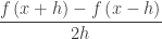
In the last post we defined the Forward Difference Quotient (FDQ) and the Backward Difference Quotient (BDQ). The average of the FDQ and the BDQ is called the Symmetric Difference Quotient (SDQ):

\displaystyle \frac{f\left( x+h \right)-f\left( x-h \right)}{2h}

You may be forgiven if you think this might be a better expression to use to find the derivative. It has its advantages. In fact, this is the expression used in many calculators to compute the numerical value of the derivative at a point; in calculators it is called nDeriv. Usually, it works pretty well. But if you try to find the derivative of the absolute value of x at x = 0 it will tell you the derivative is 0, which is wrong. The absolute value function is not locally linear at the origin and has no derivative there.

What went wrong?  Read the expression above. The numerator is the difference of the function values at the same distance, h, on both sides of x. Since, for the absolute value function with x = 0, these values are the same, their difference is 0. The SDQ never looks at x = 0 and doesn’t realize there is no derivative there. Thus, the limit of the SDQ is not the derivative.

This problem does not occur with the definition of derivative, since for that limit to exist the limits as h approaches zero from both sides must be equal. For the absolute value function the limit from the left is –1 and the limit from the right is +1 and therefore there is no limit and no derivative there.

Since most functions we will consider are differentiable, most of the time the SDQ and nDeriv are okay to use.

Seeing Difference Quotients Converge

This is an activity to see difference quotients graphically. Use a graphing calculator or a graphing program on a computer. One with a slider feature is better although I’ll also tell you how to use a calculator without this feature.

  1. Enter the function you want to consider as Y1 in your calculator or give it a name if you are using a computer. This is so later you can change the function without having to re-enter the next three equations.
  2. Enter the FDQ as Y2 using Y1 as the function. See Figure 1 below.
  3. Enter the BDQ as Y3 again using Y1 as the function.
  4. Enter the SDQ as Y3 again using Y1 as the function.
  5. Either set up a slider for h or go to the home screen and store a value for h. In the latter case you will have to return to the home screen and change the values.

Now graph all four functions. As you change the values of h with the slider or from the home screen, you should see three similar graphs (the difference quotients) along with the first function you entered. As h approaches zero, the three similar graphs should come together (converge) on the graph of the derivative. See Figures 2 and 3 below.

Change the first function. Some good functions to try are y = x– 4x, y = x3/3, y = sin(x) and don’t forget y = |x|. Try guessing the equation of the derivative.

Figure 2 Shows y = x3/3 in Black with the three difference quotients, h is about 2.

Figure 3 shows the same graph with h almost 0; the three difference quotients, now almost on top of each other, are closing in on the derivative.

Here is a link to a Desmos demonstration of the three difference quotients

Difference Quotients I

Difference Quotients & Definition of the Derivative

In the second posting on Local Linearity II, we saw that what we were doing, finding the slope to a nearby point, looked like this symbolically:

\displaystyle \frac{f\left( x+h \right)-f\left( x \right)}{h}

This expression is called the Forward Difference Quotient (FDQ). It kind of assumes that h > 0.

There is also the Backwards Difference Quotient (BDQ):

\displaystyle \frac{f\left( x \right)-f\left( x-h \right)}{h}=\frac{f\left( x-h \right)-f\left( x \right)}{-h}

The BDQ also kind of assumes that h > 0. If h < 0 then the FDQ becomes the BDQ and vice versa. So these are really the same thing. The limit (if it exists) as h approaches zero is the slope of the tangent line at whatever x is and this is important enough to have its own name. It is called the derivative of f at x with the notation (among others) {f}'\left( x \right) :

\displaystyle {f}'\left( x \right)=\underset{h\to 0}{\mathop{\lim }}\,\frac{f\left( x+h \right)-f\left( x \right)}{h}

Since h must approach 0 from both sides, this expression incorporates the FDQ and the BDQ in one expression.

To emphasize that h is a “change in x” this limit is often written

\displaystyle {f}'\left( x \right)=\underset{\Delta x\to 0}{\mathop{\lim }}\,\frac{f\left( x+\Delta x \right)-f\left( x \right)}{\Delta x}

The Derivative II

(In this activity I am paraphrasing and expanding the suggestions of Alan Lipp in a posting “Derivatives of Trig Functions” August 29, 2012 to the Calculus Electronic Discussion Group.)

This activity parallels the one in my last post here using technology.

    1. Enter the function you are investigating as Y1 in your calculator. Later you will change this to other functions but will not have to change the following entries.  Start with Y1 = x2.
    2. Enter

      \displaystyle Y2=\frac{Y1(x+0.0001)-Y1(x)}{0.0001}.

      This will approximate the derivative. This expression is called the forward difference quotient.

    1. Graph in a square window.
    1. Guess the equation of the graph you see for Y2, enter you guess in Y3 and graph it. If your guess is correct what should you see?
    1. Deselect Y1 and produce a table for the Y2 and Y3 graph. Do the values of Y2 look like what you guessed for Y3? If not, adjust your guess for Y3. (Hint: because Y2 is an approximation, they will be close but not exact.)
  1. Another way to check your guess is to graph Y4 = Y2/Y3. If your guess is close, Y4 should be the line y = 1. If their guess is wrong, the graph of Y4 may give a clue as to the correct answer. If the guess the derivative of x2 is x, then Y4 = 2 hinting that the correct guess is 2x.

A comment: Calculators have a built in numerical derivative function usually called nDeriv or d/dx. You may use this in step 2 above. However, entering and using the expression for the approximate derivative as above, reinforces the concept and is more transparent for the student than using some strange new built-in function.

Now repeat the exercise above with other functions. Chose functions whose derivatives are easy to guess for example, y = x3, y = x4, y = x5, etc., and  y = sin(x), and y = cos(x).

Keep a list of the results, so you can check it later.

The Derivative I

In “Local Linearity II”, my post for August 31, 2012, we developed a way of approximating the slope of a function at any point. The slope at x = a is approximated by

\displaystyle \frac{f\left( a+h \right)-f\left( a \right)}{h}

For small values of h.

The smaller the better, which suggests limits.

The limit of this expression as h approaches zero is called the derivative of f at x = a denoted by {f}'\left( a \right):

\displaystyle \ {f}'\left( a \right)=\underset{h\to 0}{\mathop{\lim }}\,\frac{f\left( a+h \right)-f\left( a \right)}{h}

Now give your students a simple function like y = x2 and give each student a different point in the interval [–4, 4] (include some fractions). Have them calculate the approximate slope and/or the derivative for their point. For each student’s value, plot on a graph the point (their a, slope at their a). Discuss the results. Guess the equation of the graph.

Of course, the result should look like the line y = 2x.  That is, the derivatives at various points, taken together, appear to be a function in their own right.

Repeat this exercise with the function y = sin(x). Guess the equation of the derivative.

We will look at this some more in the next post.

Show me the Math!

Is God a Mathematician? by Mario Livio begins

When you work in cosmology … one of the facts of life becomes the weekly letter, e-mail, or fax from someone who wants to describe to you his own theory of the universe (yes, they are invariably men). The biggest mistake you can make is to politely answer that you would like to learn more. This immediately results in an endless barrage of messages. So how can you prevent the assault? The particular tactic I found to be quite useful (short of the impolite act of not answering at all) is to point out the true fact that as long as his theory is not precisely formulated in the language of mathematics, it is impossible to assess its relevance. This response stops most amateur cosmologists in their tracks. … Mathematics is the solid scaffolding that holds together any theory of the universe.

Is God a Mathematician? discusses the question of whether mathematics was invented or discovered. Dr. Livio’s other popular books include The Accelerating Universe (cosmology), The Golden Ratio: The Story of Phi, the World’s most Astounding Number, and The Equation that Couldn’t be Solved: How Mathematical Genius Discovered the Language of Symmetry. All are excellent reads for teachers and students.