Parametric Equations and Vectors

In BC calculus the only application parametric equations and vectors is motion in a plane. Polar equations concern area and the meaning of derivatives. See the review notes for more detail and an outline of the topics. (only 3 items here)

Motion Problems: Same Thing Different Context (11-16-2012)

Implicit Differentiation of Parametric Equations (5-17-2014)

A Vector’s Derivative (1-14-2015)

Review Notes 

Type 8: Parametric and Vector Equations (3-30-2018) Review Notes

Type 9: Polar Equation Questions (4-3-2018) Review Notes

Roulettes 

This is a series of posts that could be used when teaching polar form and curves defined by vectors (or parametric equations). They might be used as a project. Hopefully, the equations that produce the graphs will help students understand these topics. Don’t let the names put you off. Except for one post, there is no calculus here.

Rolling Circles  (6-24-2014)

Epicycloids (6-27-2014)

Epitrochoids (7-1-2014) The most common of these are the cycloids.

Hypocycloids and Hypotrochoids  (7-7-2014)

Roulettes and Calculus  (7-11-2014)

Roulettes and Art – 1  (7-17-2014)

Roulettes and Art – 2 (7-23-2014)

Limaçons (7-28-2014)


The College Board is pleased to offer a new live online event for new and experienced AP Calculus teachers on March 5th at 7:00 PM Eastern.

I will be the presenter.

The topic will be AP Calculus: How to Review for the Exam:  In this two-hour online workshop, we will investigate techniques and hints for helping students to prepare for the AP Calculus exams. Additionally, we’ll discuss the 10 type questions that appear on the AP Calculus exams, and what students need know and to be able to do for each. Finally, we’ll examine resources for exam review.

Registration for this event is $30/members and $35/non-members. You can register for the event by following this link: http://eventreg.collegeboard.org/d/xbqbjz


Advertisement

Polar Equations

Ideally, as with parametric and vector functions, polar curves should be introduced and covered thoroughly in a pre-calculus course. Questions on the BC exams have been concerned with calculus ideas related to polar curves. Students have not been asked to know the names of the various curves (rose, curves, limaçons, etc.). The graphs are usually given in the stem of the problem, but students should know how to graph polar curves on their calculator, and the simplest by hand.

What students should know how to do:

  • Calculate the coordinates of a point on the graph,
  • Find the intersection of two graphs (to use as limits of integration).
  • Find the area enclosed by a graph or graphs: Area =\displaystyle A=\tfrac{1}{2}\int_{{{\theta }_{1}}}^{{{\theta }_{2}}}{(r(}θ\displaystyle ){{)}^{2}}dθ
  • Use the formulas x\left( \theta  \right)\text{ }=~r\left( \theta  \right)\text{cos}\left( \theta  \right)~~\text{and}~y\left( \theta  \right)\text{ }=~r(\theta )\text{sin}\left( \theta  \right)~  to convert from polar to parametric form,
  • Calculate \displaystyle \frac{dy}{d\theta } and \displaystyle \frac{dx}{d\theta } (Hint: use the product rule on the equations in the previous bullet).
  • Discuss the motion of a particle moving on the graph by discussing the meaning of \displaystyle \frac{dr}{d\theta } (motion towards or away from the pole), \displaystyle \frac{dy}{d\theta } (motion in the vertical direction) or \displaystyle \frac{dx}{d\theta } (motion in the horizontal direction).
  • Find the slope at a point on the graph, \displaystyle \frac{dy}{dx}=\frac{dy/d\theta }{dx/d\theta }.

This topic appears only occasionally on the free-response section of the exam instead of the Parametric/vector motion question. The most recent on the released exams were in 2007,  2013, 2014, and 2017. If the topic is not on the free-response then 1, or maybe 2 questions, probably finding area, can be expected on the multiple-choice section.

Shorter questions on these ideas appear in the multiple-choice sections. As always, look over as many questions of this kind from past exams as you can find.


Here are the few post I have written on polar curves and polar graphing.

Limaçons   A discussion of how polar curves are graphed

Back in the summer of 2014 I got interested in some polar equations and wrote a series of post on them which include some gifs showing how they are graphed. They are nothing that will appear on the AP exams. You can use them as enrichment if you like.

Rolling Circles

Roulettes and Calculus

Epitrochoids

Epicycloids

Hypocycloids and Hypotrochoids

Roulettes and Art – 1  

Roulettes and Art – 2


February 2016

As I hope you’ve noticed there is a new pull-down on the navigation bar called “Website.” For some years I’ve had a website at linmcmullin.net that lately I’ve been neglecting. I decided to close it in the next few days, and therefore, I move most of the material that is there to this new tab. The main items of interest are probably those under “Calculus”, “Winplot”, and “CAS.” If you used that website you should be able to find what you need here. If you cannot find something, then please write and I’ll try to help.

In my post entitled January 2016 are listing of post for the applications of integration for both AB and BC calculus. This month’s posts are BC topics on sequences, series, and parametric and polar equations.

Posts from past Februarys

Sequences and Series

February 9, 2015 Amortization A practical application of sequences.

February 8, 2013: Introducing Power Series 1

February 11, 2013: Introducing Power Series 2

February 13, 2013: Introducing Power Series 3

February 15, 2013 New Series from Old 1

February 18, 2013: New Series from Old 2

February 20, 2013: New Series from Old 3

February 22, 2013: Error Bounds

May 20, 2015 The Lagrange Highway

Polar, Parametric, and Vector Equations

March 15, 2013 Parametric and Vector Equations

March 18, 2013 Polar Curves

May 17, 2014 Implicit Differentiation of Parametric Equations 

A series on ROULETTES some special parametric curves (BC topic – enrichment):


Limaçons

When I first started getting interested in roulettes I began in polar form graphing limaçons. Without going into as much detail as with the roulettes, I offer just one today.

I found this Winplot illustration instructive as to how polar graphs are formed and just how the graphs work and relate to rectangular form graphs of the same functions. So this could be used as a first example, or an investigation of its own.

For my example we will consider the limaçon, or a cardioid with an inner loop, given below (using t for the usual theta, since the LaTex translator doesn’t seem to be able to handle thetas).

r\left( t \right)=1.4-2\sin \left( t \right)

In polar form {{r}_{1}}\left( t \right)=1.4 is a circle with center at the pole and radius of 1.4.This is shown in light blue in the figures.

The polar curve {{r}_{2}}\left( t \right)=2\sin \left( t \right) is a circle with center at \left( 1,\tfrac{\pi }{2} \right) and radius of 1. This is shown in orange in the figures below.

The graph in the example isr\left( t \right)={{r}_{2}}\left( t \right)-{{r}_{1}}\left( t \right)  the directed distance (length of the vector) from {{r}_{1}}\left( t \right) to {{r}_{2}}\left( t \right) and is shown by the green arrow in figures 1, 3, and 4.

The blue arrow is congruent to the green with its tail at the pole; its point traces the limaçon shown in black. (Click to enlarge.)

  •  In figure 1, the distance is positive and both arrows point in the same direction along the rotating ray.
  • In figure 2, the two circles intersect and the distance between them is zero. The limaçon goes through the origin.
  • In figure 3, the curves have changed position and the directed distance is negative. The blue arrow points in the negative direction opposite to the rotating ray drawing the inner loop.
  • In figure 4, the arrows return to pointing in the same direction, but are longer due to the fact that the distance runs from the orange circle to the far side of  the light blue circle forming the bottom outside loop

In the clip below the limaçon is drawn as the black ray rotates from 0 to 2\pi  
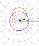
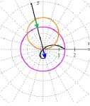
radians. Watch how the green and blue arrows (always the same length, but not the same direction), work to draw the limaçon.
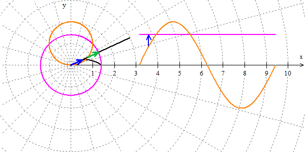
On the right side of the clip are the two functions graphed in rectangular form. The blue arrow on the right is the same length as the blue arrow on the left and gives the directed distance from {{r}_{1}}\left( t \right)  to {{r}_{2}}\left( t \right). This form is probably more familiar to students and may help them see the relationships.

A limaçon being graphed.

A limaçon being graphed.

This form is probably more familiar to students and may help them see the relationships. The Winplot file may be downloaded here. If you or your students what to investigate further, click on the Winplot graph and then CTRL+SHIFT+N to see the notes; they will also tell you how to change the A, B, and R sliders to change the curves.

Polar Curves

AP Type Questions 9

Polar Curves for BC only.

Ideally, as with parametric and vector functions, polar curves should be introduced and covered thoroughly in a precalculus course. Questions on the BC exams have been concerned with calculus ideas. Students have not been asked to know the names of the various curves (rose, curves, limaçons, etc.). The graphs are usually given in the stem of the problem, but students should know how to graph polar curves on their calculator.

What students should know how to do

  • Find the intersection of two graphs (to use as limits of integration).
  • Find the area enclosed by a graph or graphs using the formula \displaystyle A=\tfrac{1}{2}\int_{{{\theta }_{1}}}^{{{\theta }_{2}}}{(r(}θ\displaystyle ){{)}^{2}}dθ
  • Use the formulas x(θ) = r(θ)cos(θ)  and y(θ) = r(θ)sin(θ) to
    • convert from polar to rectangular form,
    • calculate the coordinates of a point on the graph, and
    • calculate \frac{dy}{d\theta } and \frac{dx}{d\theta } (Hint: use the product rule).
    • Discuss the motion of a particle moving on the graph by discussing the meaning of \frac{dr}{d\theta } (motion towards or away from the pole), \frac{dy}{d\theta } (motion in the vertical direction) or \frac{dx}{d\theta } (motion in the horizontal direction).
    • Find the slope at a point on the graph, \frac{dy}{dx}=\frac{dy/d\theta }{dx/d\theta }.

This topic appears only occasionally on the free-response section of the exam. The most recent were 2007 and 2013. If the topic is not on the free-response then 1, or maybe 2 questions, probably finding area, can be expected on the multiple-choice section.