Real “Real-life” Graph Reading

A few days ago, Paul Krugman wrote a blog about the job situation in the US.   Evan J. Romer, a mathematics teacher from Conklin, NY, used it as the basis for a great exercise on reading the graph of the derivative, the subject of my last post. He posted the questions to the AP Calculus Learning Community.  I liked them so much I have included them on my blog with Evan’s kind permission. The questions and solutions are here and on the Resources Tab above.

He used the graph below which shows the change in the number of non-farm jobs per month; in other words, the graph of a derivative of the number of people employed. The jagged graph is the data; the smooth graph is a model approximating the data.
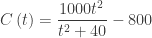
The model is \displaystyle C\left( t \right)=\frac{1000{{t}^{2}}}{{{t}^{2}}+40}-800

From this Mr. Romer developed a series of questions very similar to AP questions.  Don’t overlook the last note which discusses a “classic AP calculus mistake” made by the first person to reply to Krugman’s blog.

The first of Romer’s questions are integration questions, which you may not yet have gotten to with your class. Below is another graph of nearly the same data displayed as a bar graph. (Around February 2010 this was dubbed the “Bikini Graph” – if you look at the graph before that date you will see why.) It may be helpful in explaining the first of Romer’s questions to your class since each bar represents the change in the number of jobs for that month and leads into the concept of accumulation and the integral as the area between the graph and the axis. You can return to this when you introduce integration.

Thank You Evan.

Reading the Derivative’s Graph

A very typical calculus problem is given the equation of a function, to find information about it (extreme values, concavity, increasing, decreasing, etc., etc.). This is usually done by computing and analyzing the first derivative and the second derivative. All the textbooks show how to do this with copious examples and exercises. I have nothing to add to that. One of the “tools” of this approach is to draw a number line and mark the information about the function and the derivative on it.

A very typical AP Calculus exam problem is given the graph of the derivative of a function, but not the equation of either the derivative or the function, to find all the same information about the function. For some reason, student find this difficult even though the two-dimensional graph of the derivative gives all the same information as the number line graph and, in fact, a lot more.

Looking at the graph of the derivative in the x,y-plane it is easy to very determine the important information. Here is a summary relating the features of the graph of the derivative with the graph of the function.

Feature the function
{y}'> 0 is increasing
{y}' < 0 is decreasing
{y}' changes  – to + has a local minimum
{y}'changes + to – has a local maximum
{y}' increasing is concave up
{y}' decreasing is concave down
{y}' extreme value has a point of inflection

Here’s a typical graph of a derivative with the first derivative features marked.

Here is the same graph with the second derivative features marked.

The AP Calculus Exams also ask students to “Justify Your Answer.” The table above, with the columns switched does that. The justifications must be related to the given derivative, so a typical justification might read, “The function has a relative maximum at x-2 because its derivative changes from positive to negative at x = -2.”

Conclusion Justification
y is increasing {y}'> 0
y is decreasing {y}'< 0
y has a local minimum {y}'changes  – to +
y has a local maximum {y}'changes + to –
y is concave up {y}'increasing
y is concave down {y}'decreasing
y has a point of inflection {y}'extreme values


For notes on vertical asymptotes see

For notes on horizontal asymptotes see Other Asymptotes

Extreme Values

Every function that is continuous on a closed interval must have a maximum and a minimum value on the interval. These values may all be the same (y = 2 on [-3,3]); or the function may reach these values more than once (y = sin(x)) .

The extreme values are either (1) at an endpoint of the interval (y = 4 – 2x, on [-3, 3]), or (2) at a critical number. This is known as the Extreme Value Theorem. It is a good one to “play” with: do some sketches of the different situation above; discuss why the interval must be closed.

One way the shapes can change is if the first derivative is zero or undefined at the point where two shapes join. In this case the point is a local extreme value of the function – a local maximum or minimum value. Specifically:

  • If the first derivative changes from positive to negative, the shape of the function changes from increasing to decreasing and the point is a local maximum.  If the first derivative changes from negative to positive, the shape of the function changes from decreasing to increasing and the point is a local minimum.

This is a theorem called the First Derivative Test. By finding where the first derivative changes sign and in which direction it changes (positive to negative, or negative to positive) we can locate and identify the local extreme value precisely.

  • Another way to determine if a critical number is the location of a local maximum or minimum is a theorem called the Second Derivative Test.

If the first derivative is zero (and specifically not if it is undefined) and the second derivative is positive, then the graph has a horizontal tangent line and is concave up. Therefore, this is the location of a local minimum of the function.

Likewise, if the first derivative is zero at a point and the second derivative is negative there, the function has a local maximum there.

If both the first and second derivatives are zero at a point, then the second derivative test cannot be used, for example y = x4 at the origin.

The mistake students make with the second derivative test is in not checking that the first derivative is zero.

In the case where both the first and second derivatives are zero at the same point the function changes direction but not concavity (e.g.  (x) = xat the origin), or changes concavity but not direction (e.g. .  (x) = xat the origin).

Next: More about Concavity

Joining the Pieces of a Graph

In this post we will consider how the shapes discussed in the previous two posts can join together. Continuity and the derivative at the point where two shapes join tell us what’s going on.

Graphs can change from one shape to another only at places where:

  • The first derivative changes sign. For this to happen, the first derivative has to be either zero or undefined.  The x-coordinate at such places is called a critical number; the point is called a critical point. The function may have a local extreme value (a maximum or minimum) at its critical values. Not all critical numbers are the location of an extreme value, but all extreme values occur at critical numbers.
  • The second derivative changes sign. Such places are called a point of inflection (or, outside of the USA, point of inflexion.)  As with the first derivative, the second derivative can change sign only where it is zero or undefined. (Also, in order for there to be a second derivative at a point, the first derivative cannot be undefined there.)
  • The function is not continuous. The separate pieces can easily be different shapes. This really falls under the first bullet above, but functions may be continuous and still fail to have a derivative at a critical number.

This suggests a procedure: First, find the critical numbers by finding where {f}'\left( x \right)=0 or is undefined and then determining if there is a change of sign of the first derivative at the critical number. This may be the location of an extreme value. Compare y = x2 and y = x3 at the origin.

Do the same for points of inflection: find where {{f}'}'\left( x \right)=0 or is undefined and determine if there is a sign change there. These places may be points of inflection. Compare y = x3 and y = x4 at the origin.

A word of caution: Some authors require a non-vertical tangent line at a point of inflection and/or that the derivative exists there. This eliminates functions like y = x1/3 which has no derivative at the origin and a vertical tangent line. I see no reason for this: if there is a point where the concavity changes, that’s a point of inflection. Still you should go with your textbook’s author. The AP exams avoid asking about this situation.

If the function is not continuous (and therefore not differentiable) at a point, then the shapes don’t join. You need to look separately on each side of the point where the function is not continuous. The missing point, the jump or step, or the vertical asymptote is the clue that there may be a change in the shape. There does not have to be a change in shape at all, but as with all discontinuities be sure to check what’s happening on both sides. .

If the function is continuous, but not differentiable at a point then the shape may, but does not have to change shape there. If this is the case, the graph is not locally linear. It may have a sharp point or just a little “kink” there. But the non-differentiability tells us that something interesting is happening there.

Next: Extreme Values

Related Rate Problems II

If you look in most textbooks for related rate questions you will find pretty much the same related rate problems: ladders sliding down walls, people walking away from lamppost, water running into or out of cone shaped tanks, etc.

Here are two somewhat different related problems you may like.

  1. A girl starts riding down an escalator at the same time a boy starts riding up a parallel escalator. The escalators are 5 meters apart, 30 meters long, and they both move at the rate of 1 m/sec.
    1. How fast is the distance between the kids changing 10 seconds later? (Answer: -1.789 m/sec.)
    2. Variation: Suppose that the girl is moving at 1 m/sec and the boy at 3 m/sec. The boy reaches the end of the escalator first and stands there. Now how fast is the distance between them changing 8 seconds after they start?  (1.486 m/sec)
    3. Variation: With the situation given in part b., write and graph a piece-wise defined function that gives the distance between the kids.  Find where this graph is continuous but not differentiable. Why does this happen? (Answer: the boy reaches the top in 10 seconds and stands still. Up to this point the distance between them is represented by a hyperbola; here it now becomes a different parabola with an abrupt change in the graph. At this point, the function is not differentiable. This second parabola appears almost linear from the 10 second point on.
  1. A 60-foot-long rope is attached to a pulley 36 feet above the ground. A lantern his attached to one end of the rope and a man holds the other end on the top of his head 6 feet off the ground. He walks away at the rate of 5 feet/sec.
    1. Find the rate at which the distance between the pulley and the top of the man’s head is changing when he is 40 feet from the point directly under the pulley? (Answer: 4 ft./sec.)
    2. Find the rate of change of the length of the man’s shadow when he is 40 feet from a point directly under the pulley? (Answer:  -0.90 ft./sec.)
    3. (Extension – extreme value problem, rather difficult) When the man starts walking the lantern is at the height of his head and his shadow is infinitely long. When is the tip of the man’s shadow closest to the point directly under the pulley and how far away is it? (Answer: At t = 3.654 sec the tip of the shadow is 39.658 feet from the point under the pulley.)

These two questions are from Audrey Weeks’ Calculus in Motion. This is a really good package of dynamic illustrations of calculus concepts and AP Exams free-response question that runs on Geometer’s Sketchpad. For more information click here. The related rate sections include both standard and non-standard problems.

Corrections made September 17, 2014, March 6, 2022