August

This note will stay on top for a while

New posts will appear below. 

Today this blog is one year old. Thanks to all of you who have been following it. I hope you have found things here that help you and your students. During the first year I gave suggestions on teaching the content of a first-year calculus course. This does not change much from year to year so the post are still here and can be found using the “Posts by Topic” and “Archive” links on the right side of the screen and the “Tags” cloud at the bottom of the screen. There is also a new page called “Thru the Year” at the top. Here you will find a list of the topics in order by month. I will add a month each month.

This coming year I will try to fill in with the topics I have not already posted about. Suggestions are always welcome.

I continue my un-retirement this year by returning to teaching high school AP calculus BC along with Algebra 1. That may make for some interesting posts.

Hope you enjoy the new pictures.

I hope you have a  good year; wish me luck on mine.

Looking Ahead

Well the AP calculus exams are over. I hope all your students did well.

I’ll be cutting down the number of posts for the next few months. I will try to post once a week or so when I find something interesting. Remember if you click one of the RSS feeds or the “Follow this Blog” at the bottom of the right hand column you can get the postings without coming directly here.

In August I plan to go back to teaching high school for the first time in 15 years. I will be filling in for a friend who is going on sabbatical. That should be interesting and fun.

This blog was stared in August 2012 and I tried to do post on topics that would help a few weeks ahead of when I though most people would be teaching them. So you can go through the year monthly from the archives section on the right. Starting this coming August I hope to fill in the gaps from the first year by writing on topics I missed or expanding on the previous ones.

In the meanwhile, I’ll be working on the third edition of my book Teaching AP Calculus. I hope it will be out early next year.

Hope you have  relaxing and productive summer!

No Foolin’

The number

357,686,312,646,216,567,629,137

is a prime number.

If you remove any number of digits from the left side, the resulting number is also prime.

Numbers like this are called left-truncatable primes (they must not contain any zeros). There are exactly 4259 others ( BTW, 4259 is a prime).

There are also exactly 82 right-truncatable primes; the largest is 73939133.

Then there are 15 primes that are both left- and right-truncatable. The largest is 739397.

(For more on truncatable primes click here.)

Looking Back and Ahead

This blog came about this way. I work with a group of AP mathematics teachers in about 40 schools in Arkansas. Since I could not see them all each week, about a year ago I thought to write the calculus teachers one or two e-mails each week to give them hints and advice on teaching calculus. Then it occurred to me that a blog would be easier to handle, would make past posts easier to find, and be a help (I hoped) to more than just my teachers. 

So last August I started. My plan was to do three posts a week, a schedule I have managed to stick to. Also I hoped to stay a week or two ahead of where they should be, so that what they liked could be incorporated into their lessons.

Now is the time to finish up and start reviewing. And so, having discussed reviewing for the last few weeks, I will consider my first year as completed.

For the next few months, I will probably be posting less often. I will write about whatever I think you may be interested in, or anyway whatever I find interesting.

In August, getting ready for a new school year, I plan to add to the topics I’ve already written about and fill in the gaps with topics I skipped.

I hope you will continue to follow. You can sign up by clicking on “Follow Blog via Email” on the right sidebar. You will get an e-mail when a new post is available and you will not need to come here if there is nothing new.

As always, I would like to hear from you. I would especially like suggestions about what you would like me to expound on. You may use the comment space below or write me privately at lnmcmullin@aol.com.

I hope to hear from you.

Parametric and Vector Equations

AP Type Questions 8

Particle moving on a plane for BC – the parametric/vector question.

I have always had the impression that the AP exam assumed that parametric equations and vectors were first studied and developed in a pre-calculus course. In fact many schools do just that. It would be nice if students knew all about these topics when they started BC calculus. Because of time considerations, this very rich topic probably cannot be fully developed in BC calculus. I will try to address here the minimum that students need to know to be successful on the BC exam. Certainly if you can do more and include a unit in a pre-calculus course do so.

Another concern is that most textbooks jump right to vectors in 3-space while the exam only test motion in a plane and 2-dimensional vectors.

In the plane, the position of a moving object as a function of time, t, can be specified by a pair of parametric equations x=x\left( t \right)\text{ and }y=y\left( t \right) or the equivalent vector \left\langle x\left( t \right),y\left( t \right) \right\rangle . The path is the curve traced by the parametric equations.

The velocity of the movement in the x- and y-direction is given by the vector \left\langle {x}'\left( t \right),{y}'\left( t \right) \right\rangle . The vector sum of the components gives the direction of motion. Attached to the tip of the position vector this vector is tangent to the path pointing in the direction of motion. The length of this vector is the speed of the moving object. \text{Speed }=\sqrt{{{\left( {x}'\left( t \right) \right)}^{2}}+{{\left( {y}'\left( t \right) \right)}^{2}}}

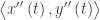
The acceleration is given by the vector \left\langle {{x}'}'\left( t \right),{{y}'}'\left( t \right) \right\rangle .

What students should know how to do

  • Vectors may be written using parentheses, ( ), or pointed brackets, \left\langle {} \right\rangle , or even \vec{i},\vec{j} form. The pointed brackets seem to be the most popular right now, but any notation is allowed.
  • Find the speed at time t\text{Speed }=\sqrt{{{\left( {x}'\left( t \right) \right)}^{2}}+{{\left( {y}'\left( t \right) \right)}^{2}}}
  • Use the definite integral for arc length to find the distance traveled \displaystyle \int_{a}^{b}{\sqrt{{{\left( {x}'\left( t \right) \right)}^{2}}+{{\left( {y}'\left( t \right) \right)}^{2}}}}dt. Notice that this is the integral of the speed (rate times time = distance).
  • The slope of the path is \displaystyle \frac{dy}{dx}=\frac{{y}'\left( t \right)}{{x}'\left( t \right)}.
  • Determine when the particle is moving left or right,
  • Determine when the particle is moving up or down,
  • Find the extreme position (farthest left, right, up or down).
  • Given the position find the velocity by differentiating; given the velocity find the acceleration by differentiating.
  • Given the acceleration and the velocity at some point find the velocity by integrating; given the velocity and the position at some point find the position by integrating. These are really just initial value differential equation problems (IVP).
  • Dot product and cross product are not tested on  the BC exam.

Shorter questions on these ideas appear in the multiple-choice sections. As always, look over as many questions of this kind from past exams as you can find.

Riemann Sums

In our last post we discussed what are called Riemann sums. A sum of the form \displaystyle \sum\limits_{i=1}^{n}{f\left( x_{i}^{*} \right)\left( {{x}_{i}}-{{x}_{i-1}} \right)} or the form \sum\limits_{i=1}^{n}{f\left( x_{i}^{*} \right)\Delta x} (with the meanings from the previous post) is called a Riemann sum.

The three most common are these and depend on where the x_{i}^{*} is chosen.

  • Left-Riemann sum, L, uses the left side of each sub-interval, so x_{i}^{*}={{x}_{n-1}}.
  • Right-Riemann sum, R, uses the right side of each sub-interval, so x_{i}^{*}={{x}_{i}}.
  • Midpoint-Riemann sum, M, uses the midpoint of each interval, so x_{i}^{*}=\tfrac{1}{2}\left( {{x}_{i-1}}+{{x}_{i}} \right).

For the AP Exams students should know these and be able to compute them. The actual values are often given in a table, so the long computation of the function values is not necessary.

Another way of approximating the area between the graph and the x-axis is to use trapezoids formed by joining the points at the ends of each sub-interval. The areas can be figured individually and added or the value, T, can be found by averaging the left- and right-Riemann sums, T=\tfrac{1}{2}\left( L+R \right). This trapezoid approximation is usually closer to the true value than the other left- or right sums.

Whenever you are dealing with approximations, you should have some sense of how good they are. All of the approximations discussed will get closer to the true area if more values (more partition points) are used.

If the graph is increasing on the interval, then the left-sum is an underestimate of the actual value and the right-sum is an overestimate.  If the curve is decreasing, then the right-sums are underestimates and the left-sums are overestimates. (To see why, draw a sketch.)

If the graph is concave up the trapezoid approximation is an overestimate, and the midpoint is an underestimate. If the graph is concave down, then trapezoids give an underestimate and the midpoint an overestimate. (To see how this works, draw a sketch. For the midpoint draw the tangent line at the midpoint to the sides of the sub-interval; this trapezoid has the same area as the rectangle drawn at the midpoint of the interval. Why?)

If the graphs are not monotone on the interval or change concavity, then all bets are off.

For all of the Riemann sums, including those not mentioned above, as the number of partition points increase (n\to \infty ), or the width of the all the sub-interval decrease (\Delta x\to 0), the limit of a Riemann sum approaches the area between the graph and the x-axis. This will be the subject of the next post.


Corrected 11-28-2017


Webinar

You might be interested in this webinar I’m leading

Wednesday December 5, 2012 at 6:30 PM Eastern Standard Time

My Favorite Function: Accumulation and Functions Defined by Integrals

Click here for the recording of this webinar.