
An existence theorem is a theorem that says, if the hypotheses are met, that something, usually a number, must exist.
For example, the Mean Value Theorem is an existence theorem: If a function f is defined on the closed interval [a, b] and differentiable on the open interval (a, b), then there exists a number c in the open interval (a, b) such that 
The phrase “there exists” also means “there is” and “there is at least one.” In fact, it is a good idea when seeing an existence theorem to reword it using each of these other phrases. “There is at least one” reminds you that there may be more than one number that satisfies the condition. The mathematical shorthand for these phrases is an upper-case E written backwards: 
- …then there is a number c in the open interval (a, b) such that…
- …then there is at least one number c in the open interval (a, b) such that…
- …then
Textbooks, after presenting an existence theorem, usually follow-up with some exercises asking you to actually find the value that exists: “Find the value of c guaranteed by the Mean Value Theorem for the function … on the interval ….” These exercises may help you remember the formula involved.
But, the important thing about most existence theorems is that the number exists, not what the number is.
Other important existence theorems in calculus
The Intermediate Value Theorem
If f is continuous on the interval [a, b] and M is any number between f(a) and f(b), then there exists a number c in the open interval (a, b) such that f(c) = M.
Another wording of the IVT: If f is continuous on an interval and f changes sign in the interval, then there must be at least one number c in the interval such that f(c) = 0
Extreme Value Theorem
If f is continuous on the closed interval [a, b], then there exists a number c in [a, b] such that 
Another wording: Every function continuous on a closed interval has (i.e. there exists) a maximum value in the interval.
If f is continuous on the closed interval [a, b], then there exists a number c in [a, b] such that 
Critical Points
If f is differentiable on a closed interval and 
Rolle’s theorem
If a function f is defined on the closed interval [a, b] and differentiable on the open interval (a, b) and f(a) = f(b), then there must exist a number c in the open interval (a, b) such that 
Mean Value Theorem – Other forms
If I drive a car continuously for 150 miles in three hours, then there is a time when my speed was exactly 50 mph.
If a function f is defined on the closed interval [a, b] and differentiable on the open interval (a, b), then there is a point on the graph of f where the tangent line is parallel to the segment between the endpoints.
Cogito, ergo sum
And finally, we have Descartes’ famous “theorem:” Cogito, ergo sum (in Latin) or in the original French, Je pense, donc je suis, translated as “I think, therefore I am” proving his own existence.


 has a (removable) discontinuity at x = 3, but no value there.
 there is no value of g(3) to use, and the derivative does not exist.
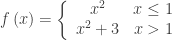 . This function has a jump discontinuity at x = 1.
 and the limit will always be a number greater than 3 divided by zero and will not exist. Therefore, even though the slopes from both side of x =1 approach the same value, namely 2, the derivative does not exist at x = 1.
 factor squeezes the function to the origin; the added condition that
  makes the function continuous. Differentiating gives
 .
. .
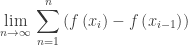
. resembles the right side of the Mean Value Theorem above. Since all the conditions are met, the MVT tells us that in each subinterval
 ![\displaystyle [{{x}_{{i-1}}},{{x}_{i}}]](https://s0.wp.com/latex.php?latex=%5Cdisplaystyle+%5B%7B%7Bx%7D_%7B%7Bi-1%7D%7D%7D%2C%7B%7Bx%7D_%7Bi%7D%7D%5D&bg=ffffff&fg=333333&s=0&c=20201002) there exists a number, call it ci , such that
there exists a number, call it ci , such that and therefore
 – The Fundamental Theorem of Calculus.)
 is called the remainder. The equation above says that if you can find the correct c the function is exactly equal to Tn(x) + R. Notice the form of the remainder is the same as the other terms, except it is evaluated at the mysterious c. The trouble is we almost never can find the c without knowing the exact value of f(x), but; if we knew that, there would be no need to approximate. However, often without knowing the exact values of c, we can still approximate the value of the remainder and thereby, know how close the polynomial Tn(x) approximates the value of f(x) for values in x in the interval, i. See
 cubic feet per hour….
 . (Which they will soon learn how to evaluate.)
 and the x-axis on the interval [2,7] and find its area =
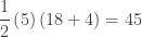
 ?” Let them think for a minute and someone will say, “Yeah, it’s
  ” And then show them

 ?”
?” ”
”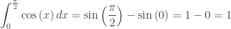

 . How much does it change from 0 to
  ? How much does it change from
  to
to  ?
?