Ideally, as with parametric and vector functions, polar curves should be introduced and covered thoroughly in a pre-calculus course. Questions on the BC exams have been concerned with calculus ideas related to polar curves. Students have not been asked to know the names of the various curves (rose, curves, limaçons, etc.). The graphs are usually given in the stem of the problem, but students should know how to graph polar curves on their calculator, and the simplest by hand.
What students should know how to do:
- Calculate the coordinates of a point on the graph,
- Find the intersection of two graphs (to use as limits of integration).
- Find the area enclosed by a graph or graphs: Area =
θ
θ
- Use the formulas
to convert from polar to parametric form,
- Calculate
and
(Hint: use the product rule on the equations in the previous bullet).
- Discuss the motion of a particle moving on the graph by discussing the meaning of
(motion towards or away from the pole),
(motion in the vertical direction) or
- Find the slope at a point on the graph,
.
This topic appears only occasionally on the free-response section of the exam instead of the Parametric/vector motion question. The most recent on the released exams were in 2007, 2013, 2014, and 2017. If the topic is not on the free-response then 1, or maybe 2 questions, probably finding area, can be expected on the multiple-choice section.
Shorter questions on these ideas appear in the multiple-choice sections. As always, look over as many questions of this kind from past exams as you can find.
Here are the few post I have written on polar curves and polar graphing.
Limaçons A discussion of how polar curves are graphed
Back in the summer of 2014 I got interested in some polar equations and wrote a series of post on them which include some gifs showing how they are graphed. They are nothing that will appear on the AP exams. You can use them as enrichment if you like.
Hypocycloids and Hypotrochoids


 changes sign.
 . The integral is the difference between whatever f represents at b and what it represents at a. (2009 AB 2 c, AB 3c, 2013 AB3/BC3 c)
 for
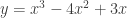
for  . Find the location of the minimum value of f(x). Justify your answer three different ways (without reference to each other).

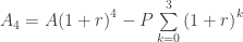
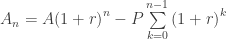
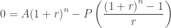
 = the original amount plus the interest on this amount minus the payment, P.
 =
=  , minus the payment, P.


 .
.
 .
. .
.
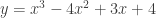
 , the count is 4 + 2 + 0 = 6. Turning points = 5
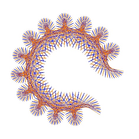
 is a circle with center at the pole and radius of 1.4.This is shown in light blue in the figures.
 is a circle with center at
  and radius of 1. This is shown in orange in the figures below.
 the directed distance (length of the vector) from
  to
to  and is shown by the green arrow in figures 1, 3, and 4.
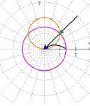
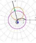

 radians. Watch how the green and blue arrows (always the same length, but not the same direction), work to draw the limaçon.
 from the first. (From the previous posts: if
  then there are d dips, loops, or cusps in n full revolutions). Both graphs will have the same R value.


 , R = 0.00667 and slightly less than a full revolution. Make the image size (under the file tab) 12.3 x 12.3 (the units are cm.), or 465 x 465 pixels (type @ after the number to use pixels). Amazing!