Definitions

Posted on August 24, 2012 by Lin McMullin

Definitions are similar to theorems, but are true in both directions; technically, this means that the statement and its converse are both true ( $p\leftrightarrow q$ ). The double arrow is read “if, and only if.” Both parts are either true or both parts are false. Definitions usually name some thing or some property. Definitions are not proved.

The definition of continuity is a good example: A function f is continuous at x = a if, and only if, these three things are true

(1) $f\left( a \right)$ exist (i.e. is a finite number)

(2) $\underset{x\to a}{\mathop{\lim }}\,f\left( x \right)$ exist (i.e. is a finite number)

(3) $\underset{x\to a}{\mathop{\lim }}\,f\left( x \right)=f\left( a \right)$ (“The limit equals the value.”)

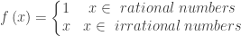
“Play” with it: consider cases where only 2 of the 3 requirements are true – is the function still continuous? What would happen if you removed the requirements about finite numbers?

To use a theorem, one must be sure all the hypotheses are true. To use a definition, one may say that either part is true once you have established that the other part is true. So, if you know a function is continuous at a point, then the three statements are true; or if you can show the three statements are true, you may say the function is continuous.

Here’s an example: A typical AP problem might give a piecewise defined function and ask if it is continuous at the place where the domain is divided.

To get credit for justifying an answer of “yes”, students must show that all the requirements of the definition are met. Specifically, they must show that the limit as x approaches that point must equal the value of the function at that point (and both are finite). In turn, to show that this limit exist the student must show that the hypotheses of the theorem that says if the two one-sided limits are equal to the same number, then that number is the limit.

To get credit for an answer of “no”, the student must show that (only) one of the hypotheses is false.

Finally, as with theorems, express definitions in words. With your students, “play” with the theorem or definition by making changes to the hypotheses and seeing how that affects the conclusion. Look at the graphs. Don’t just state the definition and expect students to understand it, remember it and use it correctly.

Theorems

Posted on August 22, 2012 by Lin McMullin

Theorems are statements that summarize the results that are true in mathematics. Theorems are statements that have been proved true; but the emphasis in AP Calculus is not on proof. Rather, it is on what the theorems mean and how to use them.

Theorems have two parts: the “if …” clause called the hypothesis and the “then …” clause called the conclusion. Students need to know both parts. In many theorems the conclusion is some sort of formula. The students need to know this, but also need to know when they can use it (the hypothesis tells them that).

An early important theorem is the Intermediate Value Theorem (IVT). Take some time with this theorem. “Play” with it. The hypothesis requires that the function be continuous on a closed interval. Use graphs (sketches, no equation needed) to show cases where the conclusion is both true and false when the function is not continuous. Can the function take on values not between f(a) and f(b)? Can you find a case where the hypothesis is met, but the conclusion is false? (Let’s hope not!)

Consider the theorem ( $p\to q$ ), its converse ( $q\to p$ ), its inverse ( $\sim p\to \sim q$ ) and its contrapositive ( $\sim q\to \sim p$ ) by looking at graphs of each case. (For the IVT the converse and inverse are false. The contrapositive of any true theorem is also true.)

Finally, for this and for all the important theorems that you use this year, express them in words, “play” with them by making change to the hypothesis, and look at graphs. Don’t just state the theorem and expect students to understand it, remember it and use it correctly.

The next post will be about definitions, which are similar to theorems in lots of ways.

For Any – For Every – For All

Posted on August 20, 2012 by Lin McMullin

The universal quantifier $\forall$ – for any – for every – for all

Many theorems and definitions in mathematics use the phrases “for any”, “for every” or “for all.” The upside-down A is the symbol. The three phrases all mean the same thing!

For example, we have the definition “A function is increasing on an interval if, and only if, for all pairs of numbers x₁ and x₂ in the interval, if x₁< x₂ then f(x₁) < f(x₂).” Whenever you have a theorem or definition with one, restating it with the other two will help students understand it better: “for all pairs of numbers,” “for any pair of numbers” and “for every pair of numbers.”

Increasing and Decreasing Functions

The symbols in the definition above tell the whole story – sure they do. As with any theorem or definition, use the Rule of Four. The definition above is the analytic part. The graphical part is the obvious – the graph goes up to the right. The numerical part is that as the x-values increase in a table, so do the y-values. The verbal part is the two preceding sentences and all the talking you’re going to have to do to explain this.

The function $y=\sin \left( x \right)$ increases on the closed interval $\left[ -\tfrac{\pi }{2},\tfrac{\pi }{2} \right]$ and the function decreases on the closed interval $\left[ \tfrac{\pi }{2},\tfrac{3\pi }{2} \right]$ . The fact that $\tfrac{\pi }{2}$ is in both intervals is not a problem since it is in the intervals, not at the point, that the function increases or decreases. This is because $\sin \left( \tfrac{\pi }{2} \right)$ is larger than all (every, any) values in $\left[ -\tfrac{\pi }{2},\tfrac{\pi }{2} \right]$ , and also larger than all (any, every) of the values in $\left[ \tfrac{\pi }{2},\tfrac{3\pi }{2} \right]$ .

“Playing” with theorems: You will soon have a theorem that says, “If the derivative of a function is positive on an interval, then the function is increasing on the interval.” Nothing in the paragraph above contradicts this, because the hypothesis says nothing about what is true if the derivative is zero. For this you have to go back to the definition. The converse of this theorem is false. Counterexample: $f\left( x \right)={{x}^{3}}$ is increasing on any (all, every) interval containing the origin, yet $f'\left( 0 \right)=0$ . The AP exams do not make a big deal of this; they accept either open or closed intervals for increasing or decreasing.

Fun with Continuity

Posted on August 17, 2012 by Lin McMullin

Most functions we see in calculus are continuous everywhere or at all but a few points that can be easily identified. But consider the Dirichlet function:

$Q\left( x \right)=\left\{ \begin{matrix} 1 & x\in \ rational\ numbers \\ 0 & x\in \ irrational\ numbers \\ \end{matrix} \right.$

Since there is one (actually many) rational numbers between any two irrational number and one (many again) irrational numbers between any two rational numbers, this function is not continuous anywhere!

But a very similar function is continuous at exactly one point (1, 1):

$f\left( x \right)=\left\{ \begin{matrix} 1 & x\in \ rational\ numbers \\ x & x\in \ irrational\ numbers \\ \end{matrix} \right.$

Can you use this idea to make a function that is continuous at exactly two points?

Asymptotes

Posted on August 15, 2012 by Lin McMullin

Horizontal asymptotes are the graphical manifestation of limits as x approaches infinity. Vertical asymptotes are the graphical manifestation of limits equal to infinity (at a finite x-value).

Thus, since $\displaystyle \underset{x\to \infty }{\mathop{\lim }}\,\left( 1-{{2}^{-x}} \right)=1$ . The graph will show a horizontal asymptote at y = 1.

Since the graph of $\displaystyle y={{2}^{-x}}\sin \left( x \right)$ approaches the x-axis as an asymptote, it follows that $\underset{x\to \infty }{\mathop{\lim }}\,\left( {{2}^{-x}}\sin \left( x \right) \right)=0$ . (The fact that this graph crosses the x-axis many times on its trip to infinity is not a concern; the axis is still an asymptote.)

Since $\underset{x\to 0}{\mathop{\lim }}\,\frac{1}{{{x}^{2}}}=\infty ,\underset{x\to {{0}^{-}}}{\mathop{\lim }}\,\frac{1}{x}=-\infty ,\text{ and }\underset{x\to {{0}^{+}}}{\mathop{\lim }}\,\frac{1}{x}=\infty$ , the functions all have a vertical asymptote of x = 0.

Continuity

Posted on August 13, 2012 by Lin McMullin

Limits logically come before continuity since the definition of continuity requires using limits. But practically and historically, continuity comes first. The concept of a limit is used to explain the various kinds of discontinuities and asymptotes. Start by studying discontinuities.

Types of discontinuities to consider: removable (a gap or hole in the graph), jump, infinite (vertical asymptotes), oscillating, and end behavior (horizontal asymptotes).

Numerically: Make a table for the value of $\displaystyle \frac{1}{x-3}$ near x = 3 and as $\displaystyle x\to \pm \infty$ . Relate the values and their signs to the graph. (Divide by a small number get a big number; divide by a big number, get a small number.)

Use the vocabulary of limits to explain the features of graphs. Example: The function $\displaystyle \frac{{{x}^{2}}-4}{x-2}$ has no value at x = 2 (f(2) does not exist), but as you get closer to x = 2 the function value gets closer to 4 ( $\displaystyle \underset{x\to 2}{\mathop{\lim }}\,f\left( x \right)=4$ ).

Relate the limit, value and graph of the function. In the example above, the graph looks like the line $y=x+2$ with a gap or hole at the point (2, 4). Another example: 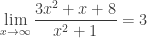$\displaystyle \underset{x\to \infty }{\mathop{\lim }}\,\frac{3{{x}^{2}}+x+8}{{{x}^{2}}+1}=3$ since, the graph gets closer to y = 3 as you go farther to the right. The line y = 3 is a horizontal asymptote.

Do this numerically as well: $\displaystyle \frac{3{{x}^{2}}+x+8}{{{x}^{2}}+1}=3+\frac{x+5}{{{x}^{2}}+1}$ and since the fraction gets smaller as |x| gets larger, the function approaches 3 from above when x > 0 and from below when x < 0 (why?)

Extra for your experts: Discuss the reason for the jump discontinuity of

$\displaystyle f\left( x \right)=\frac{\cos \left( x \right)\sqrt{{{x}^{2}}-2x+1}}{x-1}$

The Unknown Thing

Posted on August 10, 2012 by Lin McMullin

Here’s why x is so ubiquitous in mathematics.

Now one more unknown thing is known!

This TED Talk can be found here.

Teaching Calculus

The pleasure lies not in discovering the truth, but in searching for it.

Author Archives: Lin McMullin

Definitions

Theorems

For Any – For Every – For All

Fun with Continuity

Asymptotes

Continuity

The Unknown Thing

Share this:

Share this:

Share this:

Share this:

Share this:

Share this:

Share this: