 A reader recently asked me to do a post answering some questions about differential equations:
The 2016 AP Calculus course description now includes a new statement about domain restrictions for the solutions of differential equations. Specifically, EK 3.5A3 states “Solutions to differential equations may be subject to domain restrictions.” [The current 2020 CED uses the same wording in Essential Knowledge statement FUN-7.E.3] Could you write a blog post discussing (1) an example of how to determine the domain restriction; (2) speculating on whether one of the points for the differential equation on the free response will be allotted for specifying the restriction; and (3) speculating whether this concept could appear on the multiple choice and if so how.
First, let me compliment him on noticing EK 3.5A3. I overlooked it and have not seen anyone pick up on this yet. It seems to be a new item in the course description. Don’t panic. In the current 2020 CED EK FUN-7.E.3 says
A single question asking for the domain and range was asked before, but some time ago. Specifically, 2000 AB6 and 2006 AB 5 asked for the domain of the solution of a differential equation (see below for both). These are the only instances I can find that required students to find the domain of the solution.
Since 2008 many of the scoring standards included the domain, but they were not required to earn any points. These are discussed below. The domains were included in the solution, I suspect, because the standards are made public, and the readers want to publish the most complete answer.
What is required of the domain?
The generally accepted requirements are that the solution of a differential equation must be a function whose domain (1) must be an open interval, (2) on which the differential equation is true, and (3) contains the initial condition. Comments:
- The interval must be open since derivatives are not defined at the endpoints of intervals. The derivative is a two-sided limit and at an endpoint you can only approach from one side. While one-sided derivatives may be defined, they are a more burdensome requirement and not necessary.
- Practically speaking, this means that the solution may not cross a vertical asymptote or go through a point where the function is undefined; it must stay on the side where the initial condition is.
- The differential equation must be true in the sense that substituting the solution and its derivative(s) into the differential equation must result in an identity. (See 2007 AB 4(b) for practice).
- And of course, the initial condition point’s x-coordinate must be in the domain.
Teachers sometimes ask why we cannot just skip over an asymptote or an undefined point. When you do this, you are then working with a piecewise function. No problems there, but consider that on the piece(s) outside the domain as described above, you could have any function you want and still meet the three requirements above.
Finding the domain.
Here are some examples. Notice that the differential equation, its solution, and the initial condition all come into consideration.
2000 AB 6: After finding the solution  , finding the domain is a pre-calculus question, requiring one to solve the simple inequality
  . The domain is
 ![\displaystyle x>\sqrt[3]{\frac{-e}{2}}](https://s0.wp.com/latex.php?latex=%5Cdisplaystyle+x%3E%5Csqrt%5B3%5D%7B%5Cfrac%7B-e%7D%7B2%7D%7D&bg=ffffff&fg=333333&s=0&c=20201002) .
.
2006 AB 5: Will be discussed below in answer to another question he asked.
2008 AB 5: The differential equation is undefined at x = 0 and the initial condition is to the right of this. So, the domain is all positive numbers.
2011 AB5/BC5: The domain is given in the stem; Time starts now and the differential equation applies “for the next 20 years”, so, 0 < x < 20
2013 AB 6: The solution is  , So the domain is all x such that x = 1 (the initial condition) and for which
  . No further simplification was given. By graphing calculator the range is about
  .
.
2013 BC 5: The solution,  , contains a vertical asymptote at x = –1. Since the initial condition is (0, –1) the domain is x > –1; the side of the asymptote containing the initial condition.
2014 AB 6: Neither the equation, nor the solution,  , has any values for which x is undefined; so, the domain is all real numbers.
2016 AB 4: The differential equation is  with f(2) = 3. The solution
  , has a vertical asymptote where the denominator is 0, namely
  , and is undefined (because of the logarithm) for
  . The largest open interval containing the initial condition is between these two values, namely
2017 AB 4: The endpoints of the domain are stated in the stem of the problem. The time t begins when the potato is removed from the oven so t > 0 and the differential equation in (c) is given for t < 10. So the domain is 0 < t < 10.
2018 AB 6: Both the differential equation and its general solution are defined for all Real numbers: 
All of these require no “calculus”- they are “find the domain” questions from pre-calculus with the concern about vertical asymptotes. There are some other considerations. A longer and far more detailed discussion of this can be found in “The Domain of Solutions to Differential Equations”, by former chief reader Larry Riddle.
I think that answers the first question my reader asked. As to his second and third questions, I guess the answer is yes. At some point students will be asked to state the domain of a differential equation. My guess is it will be a fairly easy one-point part of a free-response question. If solving the differential equation is necessary, then it seems too long for a multiple-choice question. This is all guesswork on my part; I have no knowledge of what’s on future exams.
2019 AB 4: The solution is a polynomial and there valid for all Real numbers.
2021 AB 6: The solution contains a power of e. The domain is all Real numbers.
2021 BC 4: The solution contains terms with ln(x). The domain is all x > 0.
2022 AB 5: The domain is all Real Numbers
My reader also asked about absolute value
Another question that may be related to this topic is the relevancy of the absolute value signs in the solutions to differential equations. When can they be kept in the solution, and when are they redundant?
Absolute values can really confuse kids. See my posts “Absolutely” and “Absolute Value.” Pre-calculus topics, yes, but they come back again and again.
Here are two examples about absolute values and domains:
2005 AB 6: After separating the variables and applying the initial condition we arrive at  . This is not a function; its graph is an ellipse. We cannot just write
  , since that is not a function either. With the initial condition f(1) = –1, we have
  . Then choose the half of the ellipse where y is negative
  and
and  . The domain is
  .
.
2006 AB 5. The initial value question is to solve 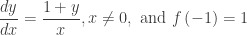 .
.
After a few steps we arrive at  . At the initial condition point
  and therefore
  . Continuing, we arrive at
  . For the AP exam, we can stop here, since we have a function and algebraic simplification is not required.
The domain was asked for. Since it is given that  , and there are no other “bad” places, the domain must be one side of the y-axis or the other. The initial condition tells us that the domain is to the left of the y-axis,
  . Since, this is so,
  and the solution simplifies to
I really appreciate questions from readers, so if you want to ask about some topic please ask me at lnmcmullin@aol.com . I’m always looking for new topics to write about – or said a different way, I’m running out of ideas!
.
Revised 4-3-18
Revised 12-23-2018 to include the 2017 and 2018 differential equation questions.
Revised 11-23-2020 – 2019 exam
Revised 1-11-2021


 .
. 
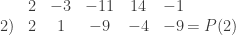

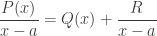

 . This is called the remainder theorem. It has a corollary called the factor theorem: If R = 0, then (x – a) is a factor of P(x).
 and substituting x = a gives
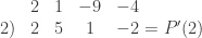
 . The value of the quotient polynomial at a is the derivative of the original polynomial at a.
 . Then
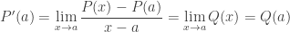


 and divide this by a:


 . Students were required to specifically state that
  somewhere, somehow, in some part of the question, showing that they understood the relationship implied by the Fundamental Theorem of Calculus.

 ; if a = 0, the series is called a Maclaurin series.
 and be able to find other series by substituting into them.
 . Re-writing a rational expression as the sum of a geometric series and then writing the series has appeared on the exam.
 θ
θ θ
θ to convert from polar to parametric form,
 and
and  (Hint: use the product rule on the equations in the previous bullet).
 (motion towards or away from the pole),
  (motion in the vertical direction) or
  .
.