The Logistic Equation

Posted on January 31, 2017 by Lin McMullin

After my last post, I realized I have never written about the logistic growth model. This is a topic tested on the AP Calculus BC exam (and not on AB). Here is a brief outline of this topic.

Logistic growth occurs in situations where the rate of change of a population, y, is proportional to the product of the number present at any time, y¸ and the difference between the number present and a number, C > 0, called the carrying capacity.

As explained in my last post, some factor limits the overall population possible to an amount C. Ask your students to sketch what they think the graph of such a function may look like and explain why.

The population starts by growing rapidly and then slows down as it approaches C. For example, if a small population of rabbits is placed on an island, the population will grow rapidly until the food starts to run out. The population will eventually level off and not grow greater than there is food to support it.

In symbols, logistic growth is modeled by the differential equation

$\displaystyle \frac{dy}{dt}=ky\left( C-y \right)$ , where k > 0 is the constant of proportionality, or by

$\displaystyle \frac{dy}{dt}=Ky\left( 1-\frac{y}{C} \right)$ and $K=Ck$

The differential equation is solved using separation of variables followed by using the method of partial fraction to obtain two expressions that can be integrated. The actual solving of the differential equation has never been tested, nor has memorization of the solution. What has been tested is what the solution graph looks like and how those features apply in real situations.

The solution, which need NOT be memorized, is $\displaystyle f\left( x \right)=\frac{C{{e}^{kCx}}}{{{e}^{kCx}}+kcD}$ (D is the constant of integration formally known as “+C.”)

The important features of the graph of the function can be found by examining the differential equation. This is an exercise consistent with MPAC 4: Connecting multiple representations and MPAC 5: Building notational fluency.

The figure above shows the slope field for a typical logistic differential equation. The values of y where $\frac{dy}{dt}=0$ indicate the location of a horizontal asymptote. There are horizontal asymptotes at y = 0 and y = C.

For points between the asymptotes $0<y<C$ , all the factors of the differential equation are positive. This indicates that the function is increasing. Near y = 0 and y = C one factor or the other is small, approaching 0: the graph of the solution (heavy blue line) is leveling off and approaching y = C from below as an asymptote. If the graph is extended into the second quadrant (thin blue line), it approaches the x-axis from above as an asymptote.

If the initial condition is greater than C then the (C – y) factor is negative, and the solution function is decreasing and approaching the asymptote y = C from above. If the number of rabbits put on the island is more than the carrying capacity, the population decreases (the poor rabbits starve).

The differential equation is a quadratic in y. Moving from the initial condition to right the slope of the tangent lines are positive and increasing, so the solution’s graph is concave upwards. After $y=\tfrac{1}{2}C$ the values of the slope (differential equation) remain positive but decrease indicating that the graph is now increasing and concave down. After this point the two factors of the differential equation switch values; that is, moving the same distance left and right of this point the product will be the same, but the values of each factor will have switched. Thus, the point where $y=\tfrac{1}{2}C$ is not only a point of inflection, but also a point of symmetry of the graph.

The maximum value occurs of the first derivative (the differential equation) is at $y=\tfrac{1}{2}C$ . This can be determined from the properties of a quadratic expression or from the second derivative,

$\displaystyle \frac{{{d}^{2}}y}{d{{t}^{2}}}=k\left( y\left( -1 \right)+\left( C-y \right)\left( 1 \right) \right)\cdot \frac{dy}{dt}=k\left( C-2y \right)\frac{dy}{dt}$ .

The second derivative is 0 at $y=\tfrac{1}{2}C$ . This is a point of inflection, the place where the function is increasing most rapidly.

Here is a Desmos demonstration that can be used to investigate the logistic differential equation, its slope field, and solution.

These ideas have all been tested on various BC exams. I cannot quote the questions here, but you may look them up for yourself.

Free-response:

2004 BC 5: (a) asymptotes as limits, and (b) when is the population growing fastest.

2008 BC 6: (a) sketch logistic equation on given slope field for two initial conditions – one between the asymptotes and one above the carrying capacity

Multiple-choice:

2003 BC 21: asymptote as a limit

2008 AB 22: Even though not an AB topic, the translation from words to symbols of the logistic model was tested on the 2008 AB multiple-choice exam. The idea was the translating, not knowledge of the logistic model.

2008 BC 24 given graph, identify differential equation.

2012 BC 14 identify logistic differential equation

There are also logistic questions on the restricted multiple-choice BC exams from 2013, 2014, and 2016; you’ll have to find them for yourself.

If you would like to experiment with logistic equations try graphing using Winplot for PC, Winplot for MACs, Geogebra, or some other program that will graph slope fields and solutions and has sliders. Desmos does not currently graph slope fields, but the solution graph can be produced.

For the differential equation enter $\frac{dy}{dx}=ky\left( C-y \right)$ with sliders for k and C.

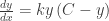
If you just want to look at the solution, use any grapher with sliders. The solution can be graphed as $\displaystyle f\left( x \right)=\frac{C{{e}^{kCx}}}{{{e}^{kCx}}+kcD}$ with D, the constant of integration, added as a third slider.

Revised and Desmos Demo link added May 12, 2022

Logistic Growth – Real and Simulated

Posted on January 24, 2017 by Lin McMullin

The logistic growth model describes situation where the growth of some population is proportional to the number present at any time and the difference between that amount and some limiting value called the “carrying capacity.”

The standard example is this: a small group of rabbits is placed on an island. The population will grow rapidly at first (like exponential growth), but eventually will level off when the food source cannot sustain any more rabbits; the island cannot ‘carry” a larger population.Before going on, ask your students to sketch a graph that shows what this model looks like.

Other things follow the same model. The spread of a disease is one, as is the cumulative sales of almost any new product.

The first graph below shows the cumulative sales of several video games. Each graph shows a typical logistic growth shape: sort of an elongated S. The sales begin rapidly and then level off near their carrying capacity.

(Source vgchatz.com)

The second graph has information on cumulative iPad sales.

(Source: The Daily Mail.com)

The top graph is the actual cumulative iPad sales. It shows a typical logistic growth shape. The smooth graph is a copy of Steve Jobs’ estimate of cumulative sales before the iPads went on sale. He clearly anticipated the logistic growth, but the actual sales ran ahead of his expectations. Both graphs seem to be headed for the same carrying capacity. The quarterly sales are graphed as a histogram at the bottom. In calculus terms, the cumulative sales graph is the integral of the quarterly sales – the accumulation of the total sales over time.

Jobs was criticized for using the graph to hide decreasing quarterly sales estimates on the right side of the graph; sales decrease, but the cumulative number keeps rising. The criticism is correct, but is not proof of any ulterior motivation by Jobs. The growth of any new product can be expected to show such a graph and sales will certainly drop after everyone who needs/wants/can’t-live-without the product has one.

Here is another recent graph.

Simulation

Here is a way to demonstrate logistic growth in your class.

A disease is introduced into a population of people (your class). At first only one person has the disease. Then it spreads in proportion to the product of the number of people who have it and the number who do not have it. Once a person has it, they are immune and cannot get it again.

Assign everyone in the class a number 1, 2, … N. (This works best for N > 20)
Use the calculator’s random number generator to produce an integer from 1 to N.
When a person’s number comes up, that person is “sick” and stands. (Of course if they’re sick maybe they should sit.)
Then continue, in each round generate as many random numbers as people standing. Those whose numbers appear for the first time stand.
Record the round number and the number of persons standing (i.e. “sick”). Graph the number standing after each round.

Here are the results with a group of 30 people:

Round	1	2	3	4	5	6	7	8	9	10	11	12	13	14	15
Standing	1	2	3	6	11	19	22	24	28	28	28	29	29	29	30

Plot the data in a suitable window

(From Teaching Calculus,3^rd edition)

Notice the very typical S-shape of the graph, the fast initial growth, and the leveling off at the end.

Look for more on the logistic equation next week.

Coming soon:

Jan 31st, The Logistic Equation
Feb 7th, Graphing Taylor Polynomials
Feb 14th, Geometric Series – Far Out

Lab-confirmed flu hospitalizations added 3-5-2018

Everyday Series

Posted on January 17, 2017 by Lin McMullin

A Square Root

Our BC friends will soon be starting to teach series. Today, to emphasize that series are all around us, I would like to discuss series that we see every day: numbers.

Long ago I was taught that no one has ever seen a “number.” Have you ever seen a four? What we see are numerals, symbols or words that represent a number. These symbols come in two types: decimals and others. The others are better described as directions for finding the decimal representation. For example, ½ tells you to divide 1 by 2, that will give the decimal 0.5.

The place-value (decimal) representation of a number is a shortcut (and a nice one) for a series that gives the value of the number. Here 4203.876 is written as a finite series, or, if you prefer, an infinite series with the remaining terms all zero.

$4203.876=4\left( {{10}^{3}} \right)+2\left( {{10}^{2}} \right)+0\left( {{10}^{1}} \right)+3\left( {{10}^{0}} \right)+8\left( {{10}^{-1}} \right)+7\left( {{10}^{-2}} \right)+6\left( {{10}^{-3}} \right)$

Repeating decimals can also be written as infinite series. The first step is to follow the “directions” and divide 23 by 99:

$\displaystyle \frac{23}{99}=0.23\overline{23}=\sum\limits_{n=1}^{\infty }{\left( 2\left( {{10}^{1-2n}} \right)+3\left( {{10}^{-2n}} \right) \right)}$

Irrational numbers are a little different. What are they anyway? Where do they go on the number line? The decimal approximations will tell us that.

I will demonstrate a way of finding the decimals with a simple example $\sqrt{2}$ . (There are many algorithms for doing this (see especially the digit-by-digit calculation), but it only applies to square roots and doesn’t really tell us what $\sqrt{2}$ means.) The approach below lets us see what is going on.

The square root of two is the number that when multiplied by itself equals 2. The sequence 1, 1.4, 1.41, 1.414, 1.4142, 1.41421, 1.414213. … gives successively better approximation to $\sqrt{2}$ .

Each successive number is found this way. At any place in the sequence the next number must one decimal place longer and end with one of the digits 0, 1, 2, 3, …, or 9.

Let’s try 6: 1.4142136² = 2.00000010642496 Too big!

So, let’s try 5: 1.4142135² = 1.99999982358225 Too small.

We’ll use the smaller one and then compute the next digit the same way: try digits until we find the largest digit that gives a square less than 2. (Or we could use the smallest digit that gives a result largest than 2; I’ll discuss that below.)

If we continue this way we will end up with a non-decreasing sequence, since putting a digit on the end always gives a slightly larger number, except for the digit zero which gives the same number. This series is also bounded (all the values are greater than 1 and less than 2). Such a series must converge to its least upper bound. For this series, the least upper bound is the number we call $\sqrt{2}$ ; the number defined as $\sqrt{2}$ .

Consider the series 2, 1.5, 1.42, 1,415, 1,4143, 1,41422, 1,414214, … in which each term has for its last digit one more than the corresponding term in the previous series above. This series is non-increasing and bounded, and, therefore, converges to its greatest lower bound, the same number $\sqrt{2}$ .

In a way, these series define $\sqrt{2}$ .

This is not a very efficient way to find values. Some irrational numbers, like π or e, cannot be found this way. But that is not the point. The point is that all numbers have a decimal representation. This decimal representation is a shorthand way of writing the finite or infinite series that converges to the number. Since we cannot write all the decimals for many numbers, the decimal form gives a series of gives better and better approximations.

So sequences and series are all around us every day.

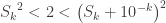
A more formal approach goes like this. Let ${{S}_{k}}$ be the k-place decimal found as described above for the first series. Then ${{S}_{k}}+{{10}^{-k}}$ will be the k-place decimal whose last digit is one more than the last digit of ${{S}_{k}}$ . Then ${{S}_{k}}^{2}<2<{{\left( {{S}_{k}}+{{10}^{-k}} \right)}^{2}}$ and ${{S}_{k}}<\sqrt{2}<{{S}_{k}}+{{10}^{-k}}$ ,. This implies $0<\sqrt{2}-{{S}_{k}}<{{10}^{-k}}$ . Since ${{10}^{-k}}$ can be made as small as we want, $\underset{k\to \infty }{\mathop{\lim }}\,\left( \sqrt{2}-{{S}_{k}} \right)=0$ and $\underset{k\to \infty }{\mathop{\lim }}\,{{S}_{k}}=\sqrt{2}$ . The series converges to $\sqrt{2}$ .

How the mind works (or at least how my mind works when it’s working):

None of this is original to me. Maybe I learned it years ago in college or graduate school; if so, I had forgotten it long ago. Four or five years ago while I was living in Texas, I started reading Calculus Deconstructed – A Second Course in First-year Calculus by Zbigniew Nitecki. He discusses this approach in a much more formal way without the example. In thinking about writing on this topic recently, I outlined the example above in my head (which is what I do when I’m trying to fall asleep). You can see where I ended up. While nothing like Nitecki’s work, it is the same idea.

I find this strange and fascinating: I absorbed that and put it all together in a different way without thinking about it in the intervening years. Strange how the mind works.

Coming soon:

Jan 24th, Logistic Growth – Real and Simulated
Jan 31st, The Logistic Equation
Feb 7th, Graphing Taylor Polynomials
Feb 14th, Geometric Series – Far Out

Density Functions

Posted on January 10, 2017 by Lin McMullin

Density, as an application of integration, has snuck onto the exams. It is specifically not mentioned in the “Curriculum Framework” chapter of the 2016 Course and Exam Description, there is one example in the 2020 CED There is an example (#12 p. 58) in the AB sample exam question section of 2020 Course and Exam Description. The first time this topic appeared was in the 2008 AB Calculus exam. There was a hint in the few years before that with a question in the old Course Description book. Both questions will be discussed below. The idea is that students are supposed to understand integration well enough to apply their knowledge to a new situation (density).

The Mathematics

A density function gives the amount of something per unit of length, area, or volume, for example

The density of a metal rod may be given in units of grams per centimeter.
The density of the population of a city may be given in units of people per square mile. (See map at end.)
The density of a container of substance may be given in pounds per cubic foot.

The density can be used to find the amount. In each example, notice that the length, area, or volume of the region is multiplied by the density to find the amount.

Example 1: A 10 cm rod with a constant density of 3 g/cm has a mass of $10\text{ cm}\cdot \frac{3\text{ grams}}{\text{cm}}=30\text{ grams}$

In other situations, the density is not constant and is given by some function. Suppose our metal rod of length b has a density of $\rho \left( x \right)$ grams/cm where x is measured from one end of the rod. To find the total mass we think of cutting the rod in the very small pieces. (Think partition: each piece has a length of $\Delta x$ in which the density is nearly constant say $\rho \left( x \right)$ .) The sum of the mass of these pieces is the Riemann sum $\sum\limits_{i=1}^{n}{\rho \left( {{x}_{i}} \right)\Delta x}$ . 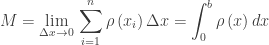The limit of this expression as $\Delta x\to 0$ gives the total mass in grams: $\displaystyle M=\underset{\Delta x\to 0}{\mathop{\lim }}\,\sum\limits_{i=1}^{n}{\rho \left( {{x}_{i}} \right)\Delta x}=\int_{0}^{b}{\rho \left( x \right)dx}$ Notice that $\sum\limits_{i=1}^{n}{\Delta x}$ is the length of the rod. This is multiplied by the density to find the mass.

Example 2: The next example is from the old Course Description book.

A city is built around a circular lake that has a radius of 1 mile. The population density of the city is $f\left( r \right)$ people per square mile, where r is the distance from the center of the lake, in miles. Which of the following expressions gives the number of people who live within 1 mile of the lake?

(A) $2\pi \int_{0}^{1}{rf\left( r \right)dr}$ (B) $2\pi \int_{0}^{1}{r\left( 1+f\left( r \right) \right)dr}$

(E) $2\pi \int_{1}^{2}{r\left( 1+f\left( r \right) \right)dr}$

We need to partition the region so that each piece has a close to a constant density. Thin rings around the lake will accomplish this. A ring, if straightened out is similar to a rectangle of length $2\pi {{r}_{i}}$ where ${{r}_{i}}$ is the distance from the center of the lake (this is the circumference of the ring), the width of this ring (rectangle) is $\Delta r$ . In this ring (rectangle) the population density is people per square mile, so the population in the ring is $f\left( {{r}_{i}} \right)$ approximated by multiplying the area by the density: $2\pi {{r}_{i}}f\left( {{r}_{i}} \right)\Delta r$ . Adding these gives a Riemann sum whose limit gives the total population:

$\underset{\Delta x\to 0}{\mathop{\lim }}\,\sum\limits_{i=1}^{n}{2\pi {{r}_{i}}f\left( {{r}_{i}} \right)\Delta r}=2\pi \int_{1}^{2}{rf\left( r \right)dr}$ Answer (D).

The limits of integration are from the edge of the lake, r = 1 to r = 2 (“one mile from the lake”). Another way to look at this is that $\sum\limits_{i=1}^{n}{2\pi {{r}_{i}}\Delta r}$ is the area of the city; this is multiplied by the population density to find the population.

This type of density situation is called a radial density function.

Notice that the answer looks like the formula for volume by cylindrical shells; this is not quite an accident. The rings around the center are like the shells used when finding volume. It is the units that are different.

Example 3: From the 2008 AB Calculus exam #92.

A city located beside a river has a rectangular boundary as shown in the figure above. The population density of the city at any point along a strip x miles from the river’s edge is $f\left( x \right)$ people per square mile. Which of the following expressions gives the population of the city?

(A) $\int_{0}^{4}{f\left( x \right)dx}$ (B) $7\int_{0}^{4}{f\left( x \right)dx}$ (C) $28\int_{0}^{4}{f\left( x \right)dx}$

(D) $\int_{0}^{7}{f\left( x \right)dx}$ (E) $4\int_{0}^{7}{f\left( x \right)dx}$

A thin vertical strip of the city ${{x}_{i}}$ miles to the right of the river has an area of $7\Delta x$ . The population in each such strip is found by multiplying the area by the density function; this gives $7f\left( {{x}_{i}} \right)\Delta x$ . These are then added forming a Riemann sum, etc.

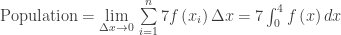
$\text{Population}=\underset{\Delta x\to 0}{\mathop{\lim }}\,\sum\limits_{i=1}^{n}{7f\left( {{x}_{i}} \right)\Delta x}=7\int_{0}^{4}{f\left( x \right)dx}$ Answer (B)

Alternative solution: When I first saw this question, not having thought about density for quite a while, I answered it by doing a unit analysis. Since unit analysis is a good thing for students to understand I’ll outline my thinking next.

We are looking for the population so the answer must be in units of “people.” The density function is in units of “people/square mile” (given). Both x and dx are in units of “miles” and the “7” also has units of “miles.” Therefore, the only choice that gives “people” is the one that multiplies the 7, the dx and the density function. This eliminates (A) and (D). The 28 in (C) must be square miles, making the overall units “people-miles” which is not what we’re going for. Finally, choice (E) is eliminated since the 7 and the dx are not in the same direction. This leaves (B).

Example 4: A volume problem adapted from Calculus by Hughes-Hallett, Gleason, et al.

The density of air h meters above the earth’s surface is $\rho \left( h \right)=1.25{{e}^{-0.00012h}}\text{ kg/}{{\text{m}}^{3}}$ . Find the mass of a column of air 25 km high with a square base 3 meters on a side sitting on the surface of the earth.

At any height, h meters above the earth the volume of a thin slice of the column of air is ${{3}^{2}}\Delta h$ . The mass of this slice is ${{3}^{2}}\rho \left( {{h}_{i}} \right)\Delta h$ . The sum of these slices gives a Riemann sum whose limit gives the total volume:

$\displaystyle M=\underset{\Delta h\to 0}{\mathop{\lim }}\,\sum\limits_{i=1}^{n}{9\rho \left( {{h}_{i}} \right)\Delta h}=9\int_{0}^{25,000}{1.25{{e}^{-0.00012h}}dh}\approx 89,082\text{ kg}\text{.}$

For other examples see 2018 BC 2, and 2021 AB 1, Good Question 15 and Good Question 16

Check the index of your textbook for density problems. Calculus by Hughes-Hallett Gleason, et al and Calculus by Rogawski (2nd edition) have good exercises and examples. My advice is not to make too big a deal of this, but if you have time, you can take a look. Should this kind of question appear on the free-response section I would guess that the question will be carefully worded so that students who never saw this kind of question would have a good chance of answering it.

The changing population density of Sydney, Australia in persons per hectare. Note the date changes in the key at the lower left.

Revised and updated 8-20-2019

Coming soon:

Jan 17th, Every Day series
Jan 24th, Logistic Growth – Real and Simulated
Jan 31st, The Logistic Equation
Feb 7th, Graphing Taylor Polynomials
Feb 14th, Geometric Series – Far Out

Definite integrals – Exam Considerations

Posted on January 3, 2017 by Lin McMullin

The sixth in the Graphing Calculator / Technology Series

Both graphing calculators and CAS calculators allow students to evaluate definite integrals. In the sections of the AP Calculus that allow calculator use students are expected to use their calculator to evaluate definite integrals. On the free-response section, students should write the integral on their paper, including the limits of integration, and then find its value on their calculator. There is no need to show the antiderivative; in fact, the antiderivative may be too difficult to find.

There are a few things students should be aware of. A question typically is worth three points: one point for the limits of integration and any constant (such as $\pi$ in a volume problem), one point for the integrand, and one point for the numerical answer. An answer alone, with no integral, may not earn any points even if it is correct.

The “Instructions” on the cover of the free-response sections read “Show your work. … Your work will be scored on the correctness and completeness of your methods as well as your answers. Answers without supporting work will usually not receive credit.” [Emphasis added] The work must be on the paper, not just on the calculator.

Another consideration is accuracy. The general directions also say, “If you use decimal approximations in calculations, your work will be scored on accuracy. Unless otherwise specified, your final answers should be accurate to three places after the decimal point.”

Let’s see how all this works in an example.

Find the area of the region between the graphs of $f\left( x \right)=x+3\cos (x)$ and $g\left( x \right)={{\left( x-2 \right)}^{2}}$ . Begin by graphing the functions and finding their points of intersections on your graphing calculator.

The values are A = 0.22532 and B = 2.41524 (or 2.41525). Students should also store these values in their calculator and recall them for the computation, as explained in a previous post. Students should write these on their paper just as shown here. Notice that a few extra decimal places should be included. The student should then show the integral and limits along with the answer on their paper:

$\displaystyle \int_{A}^{B}{\left( x-3\cos \left( x \right)-{{\left( x-2 \right)}^{2}} \right)dx=2.32651}$

Notice: Students may write A and B as the limits of integration, provided they have stated their values on the paper. This is best, but they may also write:

$\displaystyle \int_{0.22532}^{2.41525}{\left( x-3\cos \left( x \right)-{{\left( x-2 \right)}^{2}} \right)dx=2.32651}$

or even $\displaystyle \int_{0.225}^{2,415}{\left( x-3\cos \left( x \right)-{{\left( x-2 \right)}^{2}} \right)dx=2.32651}$

But be careful!!! The unrounded values should be used to do the computation. Since the limits are answers they may be rounded, but if the rounding causes the final answer to not be accurate to three places past the decimal point, then the final answer is wrong, and the answer point will not be awarded. This has happened in the past. The safest thing is to use 5 or more decimal places in your computations.

Notice also that the final answer need not be rounded as long as the first three decimal places are correct.

Teaching Calculus

The pleasure lies not in discovering the truth, but in searching for it.

Monthly Archives: January 2017

The Logistic Equation

Logistic Growth – Real and Simulated

Everyday Series

Density Functions

Definite integrals – Exam Considerations

Share this:

Share this:

Share this:

Share this:

Share this: