Stamp Out Slope-intercept Form!

Posted on January 30, 2013 by Lin McMullin

Accumulation 5: Lines

If you have a function y(x), that has a constant derivative, m, and contains the point $\left( {{x}_{0}},{{y}_{0}} \right)$ then, using the accumulation idea I’ve been discussing in my last few posts, its equation is

$\displaystyle y={{y}_{0}}+\int_{{{x}_{0}}}^{x}{m\,dt}$

$\displaystyle y={{y}_{0}}+\left. mt \right|_{{{x}_{0}}}^{x}$

$\displaystyle y={{y}_{0}}+m\left( x-{{x}_{0}} \right)$

This is why I need your help!

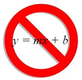
I want to ban all use of the slope-intercept form, y = mx + b, as a method for writing the equation of a line!

The reason is that using the point-slope form to write the equation of a line is much more efficient and quicker. Given a point $\left( {{x}_{0}},{{y}_{0}} \right)$ and the slope, m, it is much easier to substitute into $y={{y}_{0}}+m\left( x-{{x}_{0}} \right)$ at which point you are done; you have an equation of the line.

Algebra 1 books, for some reason that is beyond my understanding, insist using the slope-intercept method. You begin by substituting the slope into $y=mx+b$ and then substituting the coordinates of the point into the resulting equation, and then solving for b, and then writing the equation all over again, this time with only m and b substituted. It’s an algorithm. Okay, it’s short and easy enough to do, but why bother when you can have the equation in one step?

Where else do you learn the special case (slope-intercept) before, long before, you learn the general case (point-slope)?

Even if you are given the slope and y-intercept, you can write $y=b+m\left( x-0 \right)$ .

If for some reason you need the equation in slope-intercept form, you can always “simplify” the point-slope form.

But don’t you need slope-intercept to graph? No, you don’t. Given the point-slope form you can easily identify a point on the line, $\left( {{x}_{0}},{{y}_{0}} \right)$ , start there and use the slope to move to another point. That is the same thing you do using the slope-intercept form except you don’t have to keep reminding your kids that the y-intercept, b, is really the point (0, b) and that’s where you start. Then there is the little problem of what do you do if zero is not in the domain of your problem.

Help me. Please talk to your colleagues who teach pre-algebra, Algebra 1, Geometry, Algebra 2 and pre-calculus. Help them get the kids off on the right foot.

Whenever I mention this to AP Calculus teachers they all agree with me. Whenever you grade the AP Calculus exams you see kids starting with y = mx + b and making algebra mistakes finding b.

Graphing with Accumulation 2

Posted on January 28, 2013 by Lin McMullin

Accumulation 4: Graphing Ideas in Accumulation – Concavity

In the last post we saw how thinking about Riemann sum rectangles, RΣR, moving across the graph of the derivative made it easy to see when the function whose derivative was given increased and decreased and had its local extreme values. Today we will consider concavity.

Suppose a derivative is constant, its graph a horizontal line. In this case each successive RΣR is exactly the same size and adds exactly the same amount to the accumulated function. The function’s graph increases (or decreases) by exactly the same amount – it is linear.

For derivatives that are not constant, the change in the resulting function is not constant and the function’s graph bends up or down. This bending of the function is referred to as its concavity. If it bends up, the function increases faster and its graph is concave up; if it bends down, it is increasing slower (or decreasing faster) and concave down.

The graph above shows pairs of RΣR in different intervals as they move along the graph of a derivative. Consider the dark blue rectangle to be the previous position of the red rectangle.

As the RΣR moves from a to b each red rectangle is larger than the dark blue one. Each move adds more to the accumulated sum than the previous one. The graph of the function increases more with each move – it is concave up.

As the RΣR moves from b to d (there are two pairs drawn) each red RΣR has a smaller value than the previous one. (Remember when they are below the x-axis the longer (red) RΣR has a smaller value.) In the interval [b, d] less is added to the accumulated sum (or more is subtracted) with each move to the right. Therefore, the graph of the function bends down – the function is concave down.

In the last section, from d to f the red rectangle now has a larger value than the dark blue one. (Again, remember that when the function has negative values, the shorter rectangle, has the larger value.) The graph of the function again bends up – is concave up.

Putting these ideas together with those in the last post we can see how the moving RΣR idea can distinguish the four shapes of the graph of the accumulating function:

On [a, b] the function’s graph is increasing and concave up; the RΣR are positive and getting more positive (longer).

On [b, c] the function’s graph is increasing and concave down; the RΣR are positive and getting less positive (shorter).

On [c, d] the function’s graph is decreasing and concave down; the RΣR are negative and getting more negative (longer).

On [d, e] the function’s graph is decreasing and concave up; the RΣR are negative and getting less negative (shorter).

At the extreme values of the derivative, the concavity of the function changes from up to down or down to up. These are called points of inflection.

Questions in which students are asked about the properties of a function given the graph, but not the equation, of the derivative are very common. Many students (including me) find this approach easier and more intuitive than working strictly with derivative ideas.

Graphing with Accumulation 1

Posted on January 25, 2013 by Lin McMullin

Accumulation 3: Graphing Ideas in Accumulation – Increasing and decreasing

Previously, we discussed how to determine features of the graph of a function from the graph of its derivative. This required knowing (memorizing) and understanding facts about the derivative (such as the derivative is negative) and how they related to the graph of the function (the function was decreasing). There is another method that I prefer. I find that using the accumulation idea it is easy to “see” what the function is doing.

Consider the graph of the derivative of a function and picture one Riemann sum rectangle (RΣR) as it moves from left to right across the graph. If the derivative is positive the RΣR will have a positive value and if the derivative is negative the RΣR will have a negative value. Each RΣR adds to or subtracts from the accumulated value that is represented by the function.

In the drawing above we see the graph of a derivative with a RΣR drawn at three places. At a the function has some initial value which may be 0. As the RΣR moves from a to c the RΣR have a positive value and each one adds a little to the function’s value. The function accumulates value and increases.

As the RΣR moves from c to e the value of the RΣR is negative and thus subtracts from the accumulating value, so the function decreases.

In the interval e to g the RΣR once again is positive so the accumulating value increases.

At c the RΣR changes from a positive value to a negative value, the function changes from increasing to decreasing: a local maximum. A similar thing happens at e, the RΣR changes from negative to positive, the function changes from decreasing to increasing: a local minimum.

To see and determine where the function is increasing and decreasing from the graph of its derivative, just picture the RΣR sliding left to right across the graph, each one adding to or subtracting from the accumulated value which is the function.

Often there are AP Calculus exam questions that show a derivative made up of segments or parts of circles. It is possible to find the area of the regions between the derivative and the x-axis. Starting on the extreme left side add or subtract the areas of the region to find the exact function values. If the left side value is not given (that is, some other place is the initial condition), treat the left-end value as a variable and add or subtract until you get to the initial value, and solve for the variable.

Next: Accumulation and concavity

AP Accumulation Questions

Posted on January 23, 2013 by Lin McMullin

Accumulation 2: AP Exam Rate/Accumulation Questions

I assume that a number of my readers are AP Calculus teachers. In following up my last post on accumulation, today I’m going to discuss a very common type of AP Calculus exam question, the rate question which is loaded with accumulation ideas. The three posts following this one will show how accumulation can help with graphing problems.

If you do not have them, these two links will take you to them. Click on the question number for links to the question and scoring standard.

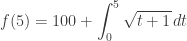
2000 AB 4: In this questions water was being pumped into a tank at the constant rate of 8 gallons per minute and leaking out at the rate of $\sqrt{t+1}$ gallons per minute. At time t = 0 we are told there are 30 gallons of water in the tank. (Many AP exams problems have two rates acting at the same time, one increasing the amount and the other decreasing it.)

The first part of the question asked for the amount of water that leaked out of the tank in the first 3 minutes. This is like the situation discussed in the last post: If you need an amount, look around for a rate to integrate. The answer is $\displaystyle\int_{0}^{3}{\sqrt{t+1}dt}=\tfrac{14}{3}\text{ gallons}\text{.}$

The next part asked for the amount of water in the tank after t minutes. So, we start with 30 gallons and add the amount put in which is 8 gallons per minute for 3 minutes of 24 gallons. Of course, we could also get this by integrating $\displaystyle \int_{0}^{3}{8dt}=24$ . Then we subtract the amount that leaked out from the first part. The amount is 30 + 24 – 14/3 gallons. This was to help students with the next part.

The third part asked for an expression for A(t), the amount of water at any time t. So following on the second part we have either $\displaystyle A\left( t \right)=30+8t-\int_{0}^{x}{\sqrt{t+1}dt}$ or $\displaystyle A\left( t \right)=30+\int_{0}^{x}{8-\sqrt{t+1}\,dt}$ . Either form, especially the latter, is the form of an accumulation function: the initial amount plus the integral of the rate of change. It was not required to actually do the integration, but if someone did then $\displaystyle A\left( t \right)=8t-\tfrac{2}{3}{{\left( t+1 \right)}^{3/2}}+\tfrac{92}{3}$

The last part asked when the maximum amount of water was in the tank. As in any extreme value problem you can find this by differentiating any of the expressions for the amount found in the third part: ${A}'\left( t \right)=8-\sqrt{t+1}$ by the FTC. (This could also be found by simply subtracting the two rates.) This will change from positive to negative when t = 63; this is when the maximum amount of water is in the tank. Notice that this is when the amount leaking out becomes greater than the amount being pumped into the tank; the total change becomes negative.

2009 AB 3: This question had a different twist or two on the accumulation idea. This proved rather difficult for the majority of the students (The mean score was 1.92 out of a possible 9 points.) The problem said that the Mighty Cable Company sold their cable for $120 per meter. The cost of producing the cable was given as $6\sqrt{x}$ dollars per meter. (Notice that these are rates as evidenced by their units $/m; the word “rate” was not used. It is important that students recognize when something is a rate.) The stem also defined profit as the difference between the amount of money received for the cable and the cost of producing the cable.

The first part of the question asked for the profit on 25 meters of cable. The amount the company receives is 25 meters times $120 dollars per meter (an amount so we could integrate the rate here, but that’s overkill). The amount the 25 meters costs to produce is (remember if you need an amount, integrate the rate): $\displaystyle \int_{0}^{25}{6\sqrt{x}\,dx}$ , so the $\displaystyle \text{Profit }=120\cdot 25-\int_{0}^{25}{6\sqrt{x}\,dx}=\$2,500$

The third part built on the first part by asking for the profit earned for a cable k meters long: $\displaystyle \text{Profit =}120k-\int_{0}^{k}{6\sqrt{x}\,dx}$ or $\displaystyle P(x)=\int_{0}^{k}{120-6\sqrt{x}\,dx}$ . There is your accumulation function. The initial value is $0.

The second part was the most interesting. In it students were asked to explain the meaning of $\displaystyle \int_{25}^{30}{6\sqrt{x}\,dx}$ in the context of the problem. One way to see what this represents is to think about the FTC. The integral of the rate in dollars per meter is the cost per meter. If we call the cost C, then $\displaystyle \int_{25}^{30}{6\sqrt{x}\,dx}=C\left( 30 \right)-C\left( 25 \right)$ . Now students did not need to do a computation here; they just have to read what the symbols mean. $C\left( 30 \right)-C\left( 25 \right)$ is the difference between the cost of manufacturing a 25-meter cable and a 30-meter table. When you integrate a rate, you get the net amount.

As in the previous question the fourth part asked for the maximum profit. This was found by differentiating the profit expression from the third part by the FTC, ${P}'\left( x \right)=120-6\sqrt{x}$ and finding when the derivative changed from positive to negative, at x = 400 meters and substituting this into the profit equation.

Accumulation: Need an Amount?

Posted on January 21, 2013 by Lin McMullin

Accumulation 1: If you need an amount, look around for a rate to integrate.

While most textbooks barely mention the word, the concept of accumulation is extremely useful in a variety of situations. This is the first of several posts will be on the topic of accumulation. We will discuss what accumulation is all about, look at some typical rate problems, discuss functions defined by integrals, see how the concept can be applied to graphing and differential equations.

The Fundamental Theorem of Calculus tells us that

$\displaystyle \int_{a}^{b}{{f}'\left( x \right)x}=f\left( b \right)-f\left( a \right)$

The integral of a rate of change (derivative) gives the net amount of change of the function over the interval. This equation tells us a lot more than just how to evaluate a definite integral. It tell us that if you are looking for the amount that something changes by, you need only integrate the rate at which it is changing: If you need an amount, integrate a rate.

So if water is pumped into a tank at the rate of $\sqrt{t+1}$ gallons per minute then the amount that is pumped in, in 5 minutes is $\displaystyle \int_{0}^{5}{\sqrt{t+1}\,dt}$ gallons. It’s as simple as that!

If a car is traveling with a velocity (rate) given by $v\left( t \right)={{t}^{2}}+6t+12$ miles per hour then the distance it travels (amount of miles) in three hours is $\displaystyle \int_{0}^{3}{{{t}^{2}}+6t+12}\,dt$ miles.

But it gets better. By changing the variables in the FTC equation a little you can write

$f\left( x \right)=f\left( a \right)+\int_{a}^{x}{{f}'\left( t \right)dt}$

This defines the function f (x) in terms of an integral whose upper limit of integration is the independent variable x. The integral gives the amount of change from t = a to t = x. This is added to the initial amount, f (a). The amount, f (x), at any time x is the initial amount, f (a), plus the amount of change between t = a and t = x, given by the integral.

If there was 100 gallons of water in the tank in the first example above, then after 5 hours there is $\displaystyle f(5)=100+\int_{0}^{5}{\sqrt{t+1}\,dt}$ gallons in the tank.

If in the second example above the car is 53 miles from its starting point and traveling in a straight line, then after 3 hours it is $\displaystyle s\left( 3 \right)=53+\int_{0}^{3}{{{t}^{2}}+6t+12}\,dt$ miles from where it started.

If you need an amount, integrate a rate.

Most Triangles Are Obtuse!

Posted on January 18, 2013 by Lin McMullin

What is the probability that a triangle picked at random will be acute? An average value problem.

The thing here is to define what you mean by picking a triangle “at random.” You could open a Geometry book and take the first triangle you come to, but are the triangles in a Geometry book really a good sample space? I doubt it.

Let’s try this: let A, B, and C be the measures, in degrees, of the angles of $\Delta ABC$ . Let A be a random number between 0 and 180, and let B be a random number between 0 and 180 – A. Then, let C = 180 – A – B.

Then $P(A<90)=\tfrac{1}{2}$

For any A < 90, B and C are chosen from the interval $\left( 0,180-A \right)$ . In order for the triangle to be acute B and C must be within 90 of both ends of this interval. That is, B and C must both be in the interval $[90-A,90]$ .

This is an interval of length A and the probability of picking numbers, B and C, at random in this interval is $\frac{A}{180-A}$ . At this point you may want to stop and calculate a typical probability. For instance, if A= 30 then the probability of both B and C being acute is $\frac{30}{180-30}=0.20$ .

In general $P\left( A<90\text{ and }\left( B<90\text{ and }C<90 \right) \right)=\frac{1}{2}\cdot \frac{A}{180-A}$ . What we need is the average of (all) these values.

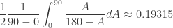
This average is $\displaystyle \frac{1}{2}\frac{1}{90-0}\int_{0}^{90}{\frac{A}{180-A}dA}\approx 0.19315$

So about 19.3% of triangles are acute, the rest are obtuse (or right). Leaving one to believe that most triangles are obtuse.

Challenge: Try writing a calculator or computer program that picks the measures of the angles of a triangle as described above. Repeat this many times while the program counts the number of acute triangles and the total number of triangles and finds their ratio. Does it come close to 19.3%?
_______________
This problem was posted on the AP Calculus Electronic Discussion Group (11/22/03) by Stu Schwartz an AP Calculus teacher at Wissahickon High School in Ambler, Pennsylvania. The solution is by one of Mr. Schwartz’s students Kurt Schneider, a tenth grader at the time who completed AB calculus in eighth grade and BC calculus in ninth grade!

Average Value of a Function

Posted on January 16, 2013 by Lin McMullin

Today I want to consider a way of developing the expression for finding the average value of a function, f (x), on an interval [a, b].

Ask students how to find the average of a bunch of numbers and they will say, “add them up and divide by the number of numbers.” Then ask if they can average an infinite number of numbers. Most will say no since you cannot divide by infinity.

Well, what if the numbers were all the same?

Such as all the y-values of f (x) = 2 between x =1 and x = 5. Isn’t the average 2? So, apparently, you can sometimes average an infinite number of numbers.

Next suggest something like f (x) = x between x = 0 and x = 3. Since half the values are obviously above 1.5 and half below, can’t 1.5 be their average? Sketch this situation and draw the segment at y = 1.5 to help them see this.

Suggest another situation, say f (x) = 2 + sin(x) on the interval $\left[ 0,2\pi \right]$ and some others. The average appears to be 2, again since half the values are above and half below 2.

When you draw the line that is the apparent average, lead the students to see that the rectangle formed by this line, the x-axis and the ends of the interval has the same area as between the function and the x-axis.

Continue with more difficult examples until someone hits on the idea of finding the “area” with an integral and then dividing the result by the width of the interval to find the height of the rectangle that is also the average value:

$\displaystyle \overline{y}=\frac{\text{''area''}}{\text{length of interval}}=\frac{\int_{a}^{b}{f\left( x \right)dx}}{b-a}$

Click here for an activity that you can use to develop this idea from scratch.

The next post: A fun application of average value – Most Triangles Are Obtuse.

Teaching Calculus

The pleasure lies not in discovering the truth, but in searching for it.

Monthly Archives: January 2013

Stamp Out Slope-intercept Form!

Graphing with Accumulation 2

Graphing with Accumulation 1

AP Accumulation Questions

Accumulation: Need an Amount?

Most Triangles Are Obtuse!

Average Value of a Function

Share this:

Share this:

Share this:

Share this:

Share this:

Share this:

Share this: