
As I wrote last week, I found an old spiral slide rule last summer. It is about the size of a rolling pin and in fact has a handle like a rolling pin’s at the bottom. The device consists of a short wide cylinder that slides around, and up or down on a longer thin cylinder.
-

- Figure 1
-

- Figure 2
The short wide cylinder has a spiral common (base 10) logarithm scale starting at the top at the 100 mark after the words “slide rule” (see Figure 3). The scale runs around the cylinder 50 times ending precisely under the starting mark. By my measurement the scale is about 511 inches or 42.6 feet long. (1.30 meters). The scale is marked for 4 digits reading with a 5th digit that can be reasonably estimated. (By way of comparison, the common 10-inch slide rule scale discussed last week allows for 2 digits reading with the third digit estimated.) These are the mantissas of the common logarithms from 1 at the zero point (since log (1) = 0) to 1.0 (log (10) = 1) at the lower end.
The thin cylinder is marked with several formulas and other information including a table of natural sines from 0 to 45 degrees, from which you can have the value of any trig function if you’re clever enough. This cylinder is not used for calculations; it is there to allow the wider cylinder to move.
There are also two pointers. The shorter one is attached to the bottom and fixed. The cylinder is moved into position for this pointer. The longer pointer is attached to the thin cylinder and can be moved to the position needed – up, down left or right. Both the top end and the bottom end of the long pointer may be used. The pointers are made to slide past each other if necessary. If the long pointer covers the number needed the other side of it may be used instead (just don’t switch back-and-forth in the same computation).
Here is how it works. For the multiplication problem 15.115 x 439.65.
For the moment we ignore the decimal points.
-

- Figure 3: Setting top marker at 1 and the first factor 1.5115.
-

- Figure 4: Setting the second factor 4.3965 and reading the product 6.645
- The top, “T” shaped, pointer is moved to the start value after “Slide rule.”
- The bottom pointer is first set at 15115 (the 151 is marked, the next 1 is the first mark following 151 and the 5 is estimated. See Figure 3 (Click to enlarge). The distance between the two measured almost 9 times around the cylinder is log (1.5115)
- Next the cylinder is moved without disturbing the pointers so that the top pointer is at 4.3965 and again estimating the last digit. Figure 4 upper long pointer.
- The product is at the fixed pointer: 6.645 Figure 4 lower pointer.
- Finally, we put the decimal in the proper place. The product is 6645.
- The full value is 6645.30975 by calculator. So the answer is correct to 4 digits, good enough for most practical work.
By moving the top pointer to log (4.3965) and using the pointers to add to it log (1.5115) we have performed the calculation log (1.5115) + log (4.3965) = log (1.5115. x 4.3965) = log (6.645)
To divide the procedure is reversed.

- Set the fixed pointer to the dividend and move the top pointer to one of the divisors. (Figure 4)
- Without moving the pointers, move the cylinder so the top pointer is at 1.
- The quotient is at the fixed pointer (Figure 3)
- Adjust the decimal point for the quotient: 15.115.
If the cylinder is moved so that the pointer is off the bottom of the cylinder, the bottom pointer is used instead of the top. (This is the reason it is directly below the top pointer.)
If this seems like a lot of trouble, it is. But remember, a working computer was not available until near the end of World War II and filled a room. Electronic calculators were not available until around 1970. Computations before then were done by hand or with logarithms.
When I was in college in the early 1960s, I worked for an engineer on my summer vacations. My boss had and occasionally used a large table of logarithms. Large, as in a whole book! As I recall, it was good without interpolating for at least 6 digits accuracy. I used a large desktop mechanical calculator that had a hand crank to do calculations. Hence the term “crank out the answer.”
As for teaching: In those old days before about 1970, you spent 3 to 4 weeks in Algebra 2 teaching students how to use logarithm table and compute with logarithms. I gave that up when the students started using calculators to do the adding and subtracting of their logarithms.
The one advantage of the spiral slide rule is that it doesn’t need batteries!
Happy Holidays!
 . I like to ask folks how many zeros this function has on the interval
  .
.
 . This is the left 10% of the first window.
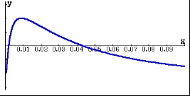


 for
for  where k is an integer, we need to see when
  . That will be when
  . And since our domain is proper fractions it must be that
  . So the zeros are infinite in number, namely
 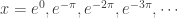 . Which answers the original question but raises others.
 . So each root is about
  of the larger next root.
 is 228.169 feet from the left edge
 is 9.860 feet from the left edge
 is 0.426 feet or 5.113 inches from the left edge
 is 0.221 inches from the left edge (less than ¼ inch)
 is about 0.134 inches from the edge.
 so its inverse will contain points of the form
  , which, since we like the first coordinate of functions to be x, we may also call
  , where ln(x) will be the name of the inverse of ex. Remember, at the moment ln(x) is just a notation for the inverse of ex, we do not know anything about logarithms (yet).
 . For example, (0, 1) is a point on eX, so (1, 0) is a point on the ln(x) function, and so ln(1) = 0.
 . Now, at
  . That is


 and the t-axis between 1 and x. If
  , then
  and if
  ,
,  .
.

 ,
,  and since ln(a) is a constant
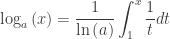
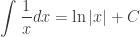 . The absolute value sign is to remind you that the argument of the logarithm function must be positive, since in some situations x itself may be negative.