Why Approximate?

Posted on October 20, 2023 by Lin McMullin

In real life everything is messier than in calculus. You are used to getting “exact” answers in mathematics. You will soon find situations where the only way to get an answer is to approximate it.

Over the year, you will learn several techniques for approximating. In college, you may take a course called Numerical Approximations, learning approximation techniques. If you use calculators or computers to find a solution; these are often approximations requiring a lot of arithmetic.

Graphing calculators approximate difference quotients using the symmetric difference quotient with a very small value of $\displaystyle \Delta x$ .

Remember when you zoomed in on a function and found that close-up it looked like a line. Over small distances near the point of tangency the tangent line has approximately the same y-coordinates as the function. This is called local linearity – over very short intervals most functions appear linear.

One way to approximate a function’s value is to travel along the tangent line from a point you know to a nearby point that you don’t know. You do this by writing the equation of the tangent line at the point you know and then moving a short distance along it. The line’s y-coordinate is close to the function’s and may be used to approximate it. Soon, when you study differential equations, you will use this idea in a slightly different way. When you get to integration and later infinite series you will learn more approximation techniques.

With any approximation, it is useful to know how close the approximation is to the value you are approximating. The first shot at this is to look at the concavity near where you are working. From the concavity you can tell if the tangent line lies above or below the curve. With that, you can determine whether you have an overestimate or an underestimate.

Now, let’s see how close we can get.

Course and Exam Description Unit 4 Section 4.6, Unit 10 Sections 10.2 and 10.10

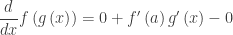
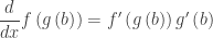
2019 CED Unit 4: Contextual Applications of the Derivative

Posted on October 7, 2019 by Lin McMullin

Unit 4 covers rates of change in motion problems and other contexts, related rate problems, linear approximation and L’Hospital’s Rule. (CED – 2019 p. 82 – 90). These topics account for about 10 – 15% of questions on the AB exam and 6 – 9% of the BC questions.

Topics 4.1 – 4.6

Topic 4.1 Interpreting the Meaning of the Derivative in Context Students learn the meaning of the derivative in situations involving rates of change.

Topic 4.2 Linear Motion The connections between position, velocity, speed, and acceleration. This topic may work better after the graphing problems in Unit 5, since many of the ideas are the same. See Motion Problems: Same Thing, Different Context

Topic 4.3 Rates of Change in Contexts Other Than Motion Other applications

Topic 4.4 Introduction to Related Rates Using the Chain Rule

Topic 4.5 Solving Related Rate Problems

Topic 4.6 Approximating Values of a Function Using Local Linearity and Linearization The tangent line approximation

Topic 4.7 Using L’Hospital’s Rule for Determining Limits of Indeterminate Forms. Indeterminate Forms of the type $\displaystyle \tfrac{0}{0}$ and $\displaystyle \tfrac{\infty }{\infty }$ . (Other forms may be included, but only these two are tested on the AP exams.)

Topic 4.1 and 4.3 are included in the other topics, topic 4.2 may take a few days, Topics 4.4 – 4.5 are challenging for many students and may take 4 – 5 classes, 4.6 and 4.7 two classes each. The suggested time is 10 -11 classes for AB and 6 -7 for BC. of 40 – 50-minute class periods, this includes time for testing etc.

Posts on these topics include:

Motion Problems

Motion Problems: Same Thing, Different Context

Speed

A Note on Speed

Related Rates

The Chain Rule

Posted on September 21, 2012 by Lin McMullin

Except for the simplest functions, a procedure known as the Chain Rule is very helpful and often necessary to find derivatives. You can start with an example such as finding the derivative of ${{\left( 2x+7 \right)}^{2}}$ . Most students will expand the binomial to get $4{{x}^{2}}+28x+49$ and differentiate the result to get $8x+28$ . They will try the same approach with ${{\left( 2x+7 \right)}^{3}}$ and then you can hit them with ${{\left( 2x+7 \right)}^{53}}$ . They will see the need for a short cut at once. What to do?

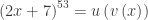
The explanation runs like this. Let $u\left( x \right)={{x}^{53}}$ and let $v\left( x \right)=2x+7$ . Then our original expression becomes ${{\left( 2x+7 \right)}^{53}}=u\left( v\left( x \right) \right)$ a composition of functions. The Chain Rule is used for differentiating compositions. Students must get good at recognizing compositions. The differentiation is done from the outside, working inward. It is done in the exact opposite order than the procedure for evaluating expression. To evaluate the expression above you (1) evaluate the expression inside the parentheses and the (2) raise that result to the 53 power. To differentiate you (1) use the power rule to differentiate the 53 power of whatever is inside, this gives $53{{\left( 2x+7 \right)}^{52}}$ , the (2) differentiate the $\left( 2x+7 \right)$ which give 2 and multiply the results: $53{{\left( 2x+{{7}^{52}} \right)}^{52}}(2)=106{{\left( 2x+7 \right)}^{52}}$ . Symbolically, this looks like ${u}'\left( v\left( x \right) \right){v}'\left( x \right)$ or ${f}'\left( g\left( x \right) \right){g}'\left( x \right)$ . This can be extended to compositions of more than two functions:

$\displaystyle \frac{d}{dx}f\left( g\left( h\left( x \right) \right) \right)={f}'\left( g\left( h\left( x \right) \right) \right){g}'\left( h\left( x \right) \right){h}'\left( x \right)$

The cartoon below is from Courtney Gibbons’ great collection of math cartoons (http://brownsharpie.courtneygibbons.org/) may help you kids remember this:

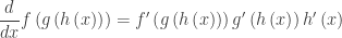
I have been looking for a way to illustrate the Chain Rule graphically, but to no avail. The closest I could come up with is this: Consider $f\left( x \right)=\sin \left( 3x \right)$ . This function takes on all the values of $y=\sin \left( x \right)$ in order in one-third the time. (That is its period is one-third of the period of $y=\sin \left( x \right)$ . Since this is true, it must go through the values three times as fast; thus, its derivative (it’s rate of change) must be three times the derivative of the sine: ${f}'\left( x \right)=3\cos \left( 3x \right)$ .

The students will need some practice on using the Chain Rule. I suggest a number of simple (single compositions) first and then a few longer ones and maybe one or two “monsters” just for fun once they get the idea.

The Chain Rule doesn’t end with just being able to differentiate complicated expressions; it will also form the basis for implicit differentiation, finding the derivative of a function’s inverse and Related Rate problems among others things.

Finally, here is a way to develop the Chain Rule which is probably different and a little more intuitive from what you will find in your textbook. (After a suggestion by Paul Zorn on the AP Calculus EDG October 14, 2002)

Let f be a function differentiable at $x=a$ , and let g be a function that is differentiable at $x=b$ and such that $g\left( b \right)=a$ . Then, near $x=a$ we can use the local linear approximation of f and g to find $\frac{d}{dx}f\left( g\left( b \right) \right)$ :

$f\left( x \right)\approx f\left( a \right)+{f}'\left( a \right)\left( x-a \right)$

$f\left( g\left( x \right) \right)\approx f\left( a \right)+{f}'\left( a \right)\left( g\left( x \right)-a \right)=f\left( a \right)+{f}'\left( a \right)g\left( x \right)-a {f}'\left( a \right)$