Good Question 2, continued.
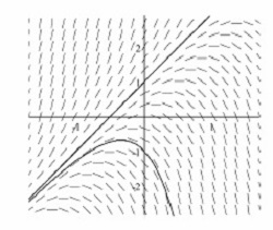
Today we continue looking at Good Question 2 from our last post. The jumping off place was the BC calculus exam question 5 from 2002. We looked at the differential equation 

The general solution of a differential equation contains a constant and therefore defines a family of functions all of whom satisfy the differential equation; they have similar, but slightly different graphs. Let’s look at and discuss the similarities and differences.
In using this with a class I suggest you present it step by step with lots of questions (more than I have here) to help them find the way to the full description of the family of functions. Alternatively, you could be very general and ask them to discuss (and justify) end behavior and the location of any extreme values or other interesting features individually or in small groups.
The Rule of Four says that all mathematical situations should be looked at analytically (i.e. with equations), graphically, numerically and verbally. In the previous post the analytic considerations were foremost and the slope field accounted for the graphical aspect. Euler’s method was numerical. Today the numerical comes to the forefront to help us discuss the graph. (Fro the verbal, well, I’ve never been accused of not being verbose, writing-wise.)
The two numbers that need to be considered are the parameter C and numerical size of e2x.
When C = 0 the solution reduces to y = 2x + 1. This is a line. If we rewrite the general solution as 
Left end behavior
Look at the x-values moving from the origin to the left; where x is negative and getting larger in absolute value. Here e2x will get very small and the solution will all get closer to the line y = 2x + 1. If C > 0 the solutions will be a little above the line and if C < 0 they will lie just below the line.
Therefore, the left end behavior is that the functions approach y = 2x + 1 as a slant asymptote.
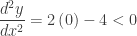
Maximum Points
In the previous post we determined that the origin was a maximum point of the solution that contained the origin (C = –1). Are there extreme points for any other solutions?
The maximums occur where 


What does this mean? It means that for all the members of the family of solutions that have C < 0 have a maximum point, and that maximum point will be on the line
Which members of the family can have maximums? Since 
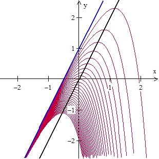
The graph above shows 30 members of the family with C = –3 (bottom curve) to C = –0.1 (top curve). The equation of the black line is y= 2x and the equation of the blue line is y= 2x + 1. Note that all the maximum points lie on the line y= 2x.
The curves with C > 0 lie above the line y= 2x + 1. For these curves

This expression will be positive when 

Therefore, all of these members of the family are concave up everywhere and since there is nowhere where their derivative is zero, there are no minimum points. See the graph below

Ten family members
from C = 0.3 (bottom curve) to C = 30 (top)
Right end behavior
From what we have determined above for C > 0 

When graphing calculators were first required on the AP calculus exams (1995) there were, for a few years, questions asking students to analyze some aspect of a family of functions. See for example 1995 BC 5, 1996 AB4/BC4, 1997 AB 4, 1997 BC 4, 1998 AB2/BC2. They seem to have stopped asking such questions. Too bad; there is some interesting calculus to be had in family of function questions.


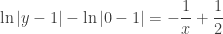
 , ignoring the –4x for the moment. This is easily solved by separating the variables
  , which can be checked by substituting.


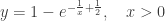
 . This may be checked by substituting. Notice that when C = 0 the particular solution is y = 2x + 1, the line through the point (0, 1).
 ) from the initial point. The first step is exactly the local linear approximation idea.

 , is found by substituting the coordinates of the previous point into the differential equation. It has the form of the equation of a line.
 with the initial point (1, 3). Approximate the value of f(2) using Euler’s method with two steps of equal size.
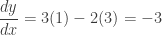 . Then
 and
and 
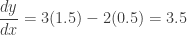
 and
and 
 . The exact value is 2.5545. A better approximation could be found using smaller steps.
 with the initial condition
  . The screen is two units wide extending from x = 0 to x = 2. The calculator graph below shows three graphs. The top graph is the particular solution
  . (I said it was easy.) The lower graph shows an approximate solution with the rather large step size of
  with the two points connected; look closely and you will see the two segments. The middle graph has a step size of
  . There are 8 segments, but they appear to be a smooth curve approximating the solution. Notice it is closer to the actual solution graph. An even smaller step size would show an even smoother graph closer to the particular solution.


 . Of course, they are not all that simple.
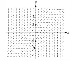
 . This is shown drawn on the slope field in the next graph. The black dot is the point (4, –3). Notice how the solution graph follows the slope field, but does not necessarily hit any of the segments. The solution will touch a segment only if the midpoint of the segment happens to be on the solution – this is not usually the case.
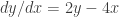 . Notice that this equation is not separable; students were not expected to solve it. They were asked to draw the solution curves through the two points (0, 1) and (0, –1) shown here in blue. These points are marked on the graph (Equa > point > (x,y)). The general solution, found by CAS, is
  , or more complicated such as
  or even more complicated.
 first appears to be
  . But we quickly realize that
  and also
  check when substituted into the given equation. In fact any equation with the form
  , where C is any constant will check. Because of this we first define the general solution of a differential equation as a function with one or more constants that satisfies the given differential equation.
 . A differential equation with an initial condition is called an initial value problem or an IVP.


 or
or  . Multiplying by 2 to simplify things, The constant in the second form is not the same as in the first. However, it is just another constant so it is okay to call it C again.
 so
so 
 and
and  with the initial condition
  . (From the 2008 AB calculus exam question 5c.)


 , so
, so  , so
, so

 . See note 2 below:
 . In order to make this so,