Why Muss with the “+C”?

Posted on June 21, 2013 by Lin McMullin

Here is a way to find the particular solution of a separable differential equation without using the +C and it might even be a little faster. As an example consider the initial value problem

$\displaystyle \frac{dy}{dx}=\frac{y-1}{{{x}^{2}}}\text{ with }x\ne 0\text{ and }y\left( 2 \right)=0$

Separate the variables as usual and then write each side a definite integral with the lower limit of integration the number from the initial condition and the upper limit variable. I’ll replace the dummy variable in the integrand with an upper-case X or Y to avoid having x and y in two places.

$\displaystyle \int_{0}^{y}{\frac{1}{Y-1}dY}=\int_{2}^{x}{{{X}^{-2}}dX}$

Integrate

$\displaystyle \left. \ln \left| Y-1 \right| \right|_{0}^{y}=\left. -{{X}^{-1}} \right|_{2}^{x}$

$\displaystyle \ln \left| y-1 \right|-\ln \left| 0-1 \right|=-\frac{1}{x}+\frac{1}{2}$

Note that near the initial condition where y = 0, $\left( y-1 \right)<0$ so $\left| y-1 \right|=-\left( y-1 \right)=1-y$ . Continue and solve for y.

$\displaystyle {{e}^{\ln \left( 1-y \right)}}={{e}^{-\frac{1}{x}+\frac{1}{2}}}$

$\displaystyle 1-y={{e}^{-\frac{1}{x}+\frac{1}{2}}}$

$\displaystyle y=1-{{e}^{-\frac{1}{x}+\frac{1}{2}}},\quad x>0$

No muss; no fuss.

Absolute Value

Posted on May 23, 2013 by Lin McMullin

The answers to the True-False quiz at the end of the last post are all false. This brings us to absolute value, another topic I want to concentrate on for my upcoming Algebra 1 class. Absolute value becomes a concern in calculus too which I will discuss as the last example below.

There a several “definitions” of absolute value that I’ve seen over the years which I mostly do not like

The number without a sign – awful: all numbers except zero have a sign
The distance from zero on the number line – true, but not too useful especially with variables
The larger of a number and its opposite – true, but not to useful with variables

So I propose to give them an algorithm: If the number is positive, then the absolute value is the same number; if the number is negative, then its absolute value is its opposite. Of course, this is really the definition.

So I’ll soon express this in symbols

$\left| a \right|=\left\{ \begin{matrix} a & \text{if }a\ge 0 \\ -a & \text{if }a<0 \\ \end{matrix} \right.$

Now interestingly this is probably the first piecewise defined function an Algebra 1 student may see, or at least the first one that’s not artificial. So this is a good place to start talking about piecewise defined function and the importance of talking about the domain. And of course, we’ll have to take a look at the graph.

Sometimes we will have to start solving equations and inequalities with absolute values. So here is the next thing I understand but do not like and will try to avoid. Solve the equation: $\left| x \right|=3$ , Answer including work: $x=\pm 3$ . But I think a longer way around is also better:

If $x<0$ then $\left| x \right|=-x=3$ so $x=-3$ or if $x>0$ , then $\left| x \right|=x=3$ Solution: $x=3$ or $x=-3$ .

Longer? Sure. I hope that by making the students write that a few times that when they get to solving $\left| x \right|>3$ that it will be natural to say

If $x<0$ then $\left| x \right|=-x>3$ so $x<-3$ or if $x>0$ , then $\left| x \right|=x>3$ Solution: $x<-3$ or $x>3$

The last case may take a little more discussion. Solve $\left| x \right|<3$ . Starting the same way

If $x<0$ then $\left| x \right|=-x<3$ so $x>-3$ which really means $-3<x<0$

if $x>0$ , then $\left| x \right|=x<3$ which really means $0\le x<3$ . Then the union of these two sets looks like an intersection. The solution is $-3<x<3$

Quite often the equation and the two types of inequalities are treated as separate problems: with = you go with $\pm$ on the other side, with > you have a union pointing away from the origin and with < you have somehow an intersection. Who needs to remember all that when this idea works all the time?

Example: Solve $\left| 4x-10 \right|<8$

If $4x-10<0$ , then $x<\tfrac{5}{2}$ and $\left| 4x-10 \right|=-\left( 4x-10 \right)=-4x+10<8$ , so $-4x<-2$ and $x>\tfrac{1}{2}$ or more precisely $\tfrac{1}{2} If$ latex 4x-10\ge 0$, then $x\ge \tfrac{5}{2}$ and $\left| 4x-10 \right|=4x-10<8$ , so $4x<18$ and $x<\tfrac{9}{2}$ or more precisely $\tfrac{5}{2}<x<\tfrac{9}{2}$ . The union again becomes an intersection and the answer is $\tfrac{1}{2}<x<\tfrac{9}{2}$

Finally an example from calculus. On the 2008 AB exam, question 5 asked student to find the particular solution of a differential equation with the initial condition $f\left( 2 \right)=0$ . After separating the variables, integrating, including the “+C” and substituting the initial condition students arrived at this equation which they now need to solve for y:

$\displaystyle \left| y-1 \right|={{e}^{\tfrac{1}{2}-\tfrac{1}{x}}}$

How can you lose the absolute value sign? Simple, near the initial condition where y = 0, $\left( y-1 \right)<0$ so replace $\left| y-1 \right|$ with $-\left( y-1 \right)$ and then go ahead and solve for y

$\displaystyle -\left( y-1 \right)={{e}^{\tfrac{1}{2}-\tfrac{1}{x}}}$

$\displaystyle y=1-{{e}^{\tfrac{1}{2}-\tfrac{1}{x}}}$

I don’t think I’ll try this one in Algebra 1, but maybe it will come in handy when they get to calculus.

Differential Equations

Posted on March 11, 2013 by Lin McMullin

AP Type Questions 6

Differential equations are tested every year. The actual solving of the differential equation is usually the main part of the problem, but it is accompanied by a question about its slope field or a tangent line approximation or something else related. BC students may also be asked to approximate using Euler’s Method. Large parts of the BC questions are often suitable for AB students and contribute to the AB subscore of the BC exam.

What students should be able to do

Find the general solution of a differential equation using the method of separation of variables (this is the only method tested).
Find a particular solution using the initial condition to evaluate the constant of integration – initial value problem (IVP).
Understand that proposed solution of a differential equation is a function (not a number) and if it and its derivative are substituted into the given differential equation the resulting equation is true. This may be part of doing the problem even if solving the differential equation is not required (see 2002 BC 5 – parts a, b and d are suitable for AB)
Growth-decay problems.
Draw a slope field by hand.
Sketch a particular solution on a (given) slope field.
Interpret a slope field.
Use the given derivative to analyze a function such as finding extreme values
For BC only: Use Euler’s Method to approximate a solution.
For BC only: use the method of partial fractions to find the antiderivative after separating the variables.
For BC only: understand the logistic growth model, its asymptotes, meaning, etc. The exams have never asked students to actually solve a logistic equation IVP.

Shorter questions on this concept appear in the multiple-choice sections. As always, look over as many questions of this kind from past exams as you can find.

For some previous posts on this subject see November 26, 2012, January 21, 2013 February 1, 6, 2013

Logarithms

Posted on February 6, 2013 by Lin McMullin

Students first encounter logarithms in Algebra 2 or their last pre-calculus course. They are usually defined as exponents and their properties “proven” by reference to the corresponding properties of exponents. This is good enough at the time, but in calculus we are ready to define logarithms properly. The result is the definition in terms of a function defined by an integral.

In fact, the definition flows naturally from the properties of inverse functions (no pun intended, because the flow is quite natural). But is this a definition? Or a proof? The solution of certain differential equations discussed in my last post may be used to derive the logarithm function.

Let’s begin by pretending we know nothing about logarithms, and investigate the inverse of e^x. (See The Derivative of Exponential Functions)

This function e^x contains points of the form $\left( X,{{e}^{X}} \right)$ so its inverse will contain points of the form $\left( {{e}^{X}},X \right)$ , which, since we like the first coordinate of functions to be x, we may also call $\left( x,\ln \left( x \right) \right)$ , where ln(x) will be the name of the inverse of e^x. Remember, at the moment ln(x) is just a notation for the inverse of e^x, we do not know anything about logarithms (yet).

So $\left( {{e}^{X}},X \right)$ = $\left( x,\ln \left( x \right) \right)$ and $X\ne x$ . For example, (0, 1) is a point on e^X, so (1, 0) is a point on the ln(x) function, and so ln(1) = 0.

In a previous post we defined the number e and the function e^x in such a way that $\displaystyle \frac{d}{dx}{{e}^{x}}={{e}^{x}}$ . Now, at $\left( X,{{e}^{X}} \right)$ the derivative is e^X, so at the corresponding point on its inverse, $\left( {{e}^{X}},X \right)$ , the derivative is the reciprocal of the derivative of e^X which is $\frac{1}{{{e}^{X}}}=\frac{1}{x}$ . That is

$\displaystyle \frac{d}{dx}\ln \left( x \right)=\frac{1}{x}$

We can use this idea to define ln(x) as a function defined by an integral. Solving the differential equation by the method suggested in a recent post we get:

$\displaystyle \ln \left( x \right)=\ln \left( a \right)+\int_{a}^{x}{\frac{1}{t}dx}$

We can pick any positive number for a and a convenient one is the one we already found a = 1 where ln(1) = 0, so

$\displaystyle \ln \left( x \right)=\int_{1}^{x}{\frac{1}{t}dx},\quad x>0$

This then is the “official definition” of the natural logarithm function. The domain is x > 0 (the range of e^x) and the range is all real numbers (the domain of e^x).

Graphically, ln(x) is the area between the graph of $\displaystyle \frac{1}{t}$ and the t-axis between 1 and x. If $0<x<1$ , then $\ln \left( x \right)<0$ and if $x>1$ , $\ln \left( x \right)>0$ .

From this definition we can prove all the familiar properties of logarithms $\left( \ln \left( ab \right)=\ln \left( a \right)+\ln \left( b \right)\text{ etc}\text{.} \right)$ and show that this is a function of the kind we called “logarithm” all along. This is in all the textbooks so I will not go into this here.

One of these properties tells us that for $a>0\text{ and }a\ne 1$ , $\displaystyle {{\log }_{a}}\left( x \right)=\frac{\ln \left( x \right)}{\ln \left( a \right)}$ and since ln(a) is a constant

$\displaystyle {{\log }_{a}}\left( x \right)=\frac{1}{\ln \left( a \right)}\int_{1}^{x}{\frac{1}{t}dt}$

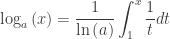
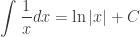
Finally, you will see this antiderivative formula: $\displaystyle \int_{{}}^{{}}{\frac{1}{x}dx=\ln \left| x \right|+C}$ . The absolute value sign is to remind you that the argument of the logarithm function must be positive, since in some situations x itself may be negative.

Revised slightly 8-28-2018

Accumulation and Differential Equations

Posted on February 1, 2013 by Lin McMullin

Accumulation 6: Differential equations

When students first learn about antiderivatives, they are given simple initial value problems to solve such as $\frac{dy}{dx}=3-2x,\quad y\left( 1 \right)=-5$ . They are instructed to find the antiderivative, then tack on a +C , then substitute in the initial condition, then solve for C and finally write the particular solution. So we hope to see:

$\frac{dy}{dx}=3-2x$

$y=3x-{{x}^{2}}+C$

$-5=3(1)-{{1}^{2}}+C$

$-7=C$

$y=3x-{{x}^{2}}-7$

But thinking of it as an accumulation problem you can write

$\displaystyle y=-5+\int_{1}^{x}{3-2t\,dt}$

$y=-5+\left. \left( 3t-{{t}^{2}} \right) \right|_{1}^{x}$

$y=-5+\left( 3x-{{x}^{2}} \right)-\left( 3(1)-{{1}^{2}} \right)$

$y=3x-{{x}^{2}}-7$

Now I’ll admit there is not too much difference in the amount of work involved there, but once the first line is on the paper there is not much to remember in what to do from there on. Common student mistakes in the first method include entirely forgetting the +C and not using the initial condition correctly.

A differential equation in which dy/dx can be written as a function of x only, $\frac{dy}{dx}={f}'\left( x \right)$ , with an initial condition $\left( a,f\left( a \right) \right)$ has the solution

$\displaystyle f\left( x \right)=f\left( a \right)+\int_{a}^{x}{{f}'\left( t \right)dt}$

Look familiar? Yes, that’s my favorite accumulation equation.

Furthermore, if all you need is some function values, this expression can be entered into a graphing calculator and the values calculated without finding an antiderivative.

In my first post on accumulation, I discussed the AP exam question 2000 AB 4. The solution to part (a) looks like this

$\displaystyle \int_{0}^{3}{\sqrt{t+1}dt}=\left. \tfrac{2}{3}{{\left( t+1 \right)}^{3/2}} \right|_{0}^{3}=\tfrac{2}{3}\left( {{4}^{3/2}}-{{0}^{3/2}} \right)=\tfrac{14}{3}\text{ gallons}$