vector equations. vector curves

Parametric and vector-valued functions are a way of writing and graphing more complicated, and therefore more interesting, curves.

Up to now you have been studying functions where the y-coordinates are found evaluating an expression in terms of the x-coordinates. Parametric and vector equations define both the x– and y-coordinates of a curve in terms of a third variable called a parameter, usually represented by t.

The only difference between the parametric and vector representation is the notation. The parametric form gives two equations, one for x and one for y. For example:

$\displaystyle x\left( t \right)=t-1.2\sin (t)$

$\displaystyle y(t)=1-1.2\cos \left( t \right)$

are the parametric equations of a curve called a prolate cycloid. It is the path of a point on the flange of a train wheel as it rolls along a straight track.

The vector form for this same curve is written:

$\displaystyle \left\langle {t-1.2\sin \left( t \right),1-1.2\cos \left( t \right)} \right\rangle$ .

Notice the two coordinates of the vector are the same as the parametric equations.

In BC calculus you will study parametric and vector-valued equations of motion, that is the path of a point moving according to the parametric and vector equation. Since things are moving, they have a velocity – a vector pulling the point in the direction it is moving at any instant. The velocity vector is tangent to the curve and its length is the speed at which the point is moving. Also, they have an acceleration – a vector pulling the velocity vector. These are found, as I hope you suspect, by differentiating. Vector-valued functions may also be integrated.

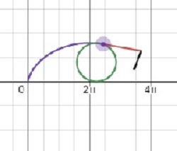
The illustration shows the path of a point on the flange of a train wheel rolling along a track. Notice that sometimes the point is moving backwards! The Position vector (from the origin to the point) is in black. Its endpoint is the point defined by the parametric or vector equations. The red vector is the velocity vector “pulling” the point to its next position. The green vector is the acceleration vector “pulling” the velocity vector.

While there are many other uses for parametric and vector-valued functions, the BC Calculus Exam only considers motion situations.

Course and Exam Description Unit 9, Sections 9.1 to 9.6. This is a BC only topic.

As you probably realize by now, I think graphs, drawing and other visuals are a great aid in teaching and learning mathematics. Desmos is a free graphing app that many teachers and students use to graph and make other illustrations. Demonstrations can be made in advance and shared with students and other teachers.

Recently, I was looking a some material from Unit 9 Parametric Equation, Polar Coordinates, and Vector-Valued Functions, BC topics, from the current AP Calculus CED. I ended up making three new Desmos illustrations for use in this unit. They will also be useful in a precalculus course introducing these topics. Hope you find them helpful.

Polar Graph Demo

Link

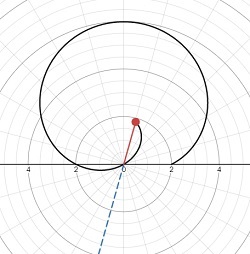
You may replace the polar equation with any polar equation you are interested in. There are directions in the demo. Moving the “a” slider will show a ray rotating around the pole. The “a” value is the angle, $\displaystyle \theta$ , in radians between the ray and the polar axis. On the ray is a segment with a point at its end. This segment’s length is $\displaystyle \left| {r\left( \theta \right)} \right|$ . As you rotate the ray you can see the polar graph drawn. When $\displaystyle r(\theta )<0$ the segment extend in the opposite direction from the ray.

This demo may be used to introduce or review how polar equation work. An interesting extension is to enter something for the argument of the function that is not an integer muntiple of $\displaystyle \theta$ and extend the domain past $\displaystyle 2\pi$ , for example $\displaystyle r=2+4\sin (1.2\theta )$

Basic Parametric and Vector Demo

LInk

A parametric equation and the vector equation of the same curve differ only in notation. So, this demo works for both. Following the directions in the demo, you may see the graph being drawn using the “a” slider. You may turn on (1) the position vector and its components, (2) add the velocity vector attached to the moving point and “pulling” it to its new position, and (3) the acceleration vector “pulling” the velocity vector.

You may enter any parametric/vector equation. When you do, you will also have to enter its first and second derivative. Follow the directions in the demonstration.

Cycloids and their vectors

Link

This demo shows the path on a rolling wheel called a cycloid. The “a” slider moves the position of the point on the wheel. The point may be on the rim of the wheel ( $\displaystyle a=r$ , on the interior of the wheel ( $\displaystyle a<r$ ), or outside the wheel ( $\displaystyle a>r$ – think the flange on a train wheel). Use the “u” slider to animate the drawing. The velocity and acceleration vectors are shown; they may be turned off. The velocity vector is tangent to the curve (not to the circle) and seems to “pull” the point along the curve. The acceleration vector “pulls” the velocity vector. The equation in this demo should not be changed.