
At an APSI this summer the participants and I got to discussing the “tabular method” for integration by parts. Since we were getting far from what is tested on the BC Calculus exams, I ended the discussion and said for those that were interested I would post more on the tabular method this blog going farther than just the basic set up. So here goes.
Here are some previous posts on integration by parts and the tabular method
Integration by Parts 1 discusses the basics of the method. This is as far as a BC course needs to go.
Integration by Parts 2 introduces the tabular method
Modified Tabular Integration presents a very quick and slick way of doing the tabular method without making a table. This is worth knowing.
There is also a video on integration by parts here. Scroll down to “Antiderivatives 5: A BC topic – Integration by parts.” The tabular method is discussed starting about time 15:16. There are several ways of setting up the table; one is shown here and a slightly different way is in the Integration by Parts 2 post above. There are others.
Going further with the tabular method.
The tabular method works well if one of the factors in the original integrand is a polynomial; eventually its derivative will be zero and you are done. These are shown in the examples in the posts above and Example 1 below. To complete the topic, this post will show two other things that can happen when using integration by parts and the tabular method.
First we look at an example with a polynomial factor and learn how to stop midway through. Why stop? Because often there will be no end if you don’t stop. There are ways to complete the integration as shown in the examples.
Example 1: Find 

Adding the last column gives the antiderivative:

Now say you wanted to stop after 

The integrand on the right is the product of the last column in the row at which you stopped and the first two columns in the next row, as shown in yellow above.
Example 2 Find


As you can see things are just repeating the lines above sometimes with minus signs. However, if we stop on the third line we can write:

The integral at the end is identical to the original integral. We can continue by adding the integral to both sides:

Finally, we divide by 2 and have the antiderivative we were trying to find:

In working this type of problem you must be aware of that the original integrand showing up again can happen and what to do if it does. As long as the coefficient is not +1, we can proceed as above. The same thing happens if we do not use the tabular method. (If the coefficient is +1 then the other terms on the right will add to zero and you need to make different choices for u and dv.)
Reduction Formulas.
Another use of integration by parts is to produce formulas for integrals involving powers. An integral whose integrand is of less degree than the original, but of the same form results. The formula is then iterated to continually reduce the degree until the final integral can be integrated easily.
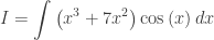
Example 3: Find

Let


This is a reduction formula; the second integral is the same as the first, but of lower degree. Here is how it is used. At each step the integrand is the same as the original, but one degree lower. So the formula can be applied again, three more times in this example.

Most textbooks have a short selection of reduction formulas.
Final Thoughts.
Back in the “old days”, BC (before calculators), beginning calculus courses spent a lot of time on the topic of “Techniques of Integration.” This included integration by parts, algebraic techniques, techniques known as trig-substitutions, and others. Mathematicians and engineers had tables of integrals listing over a thousand forms and students were taught how to use the tables and distinguish between similar forms in the tables. (See the photo below from the fourteenth edition of the CRC tables (c) 1965.) Current textbooks often contain such sections still.
Today, none of this is necessary. CAS calculators can find the antiderivatives of almost any integral. Websites such as WolframAlpha are also available to do this work.
I’m not sure why the College Board recently expanded slightly the list of types of antiderivatives tested on the exams. Certainly a few of the basic types should be included in a course, but what students really need to know is how to write the integral appropriate to a problem, and what definite and indefinite integrals mean. This, in my opinion, is far more important than being able to crank out antiderivatives of increasingly complicated expressions: let technology do that – or buy yourself an integral table. Just saying … .

 and
and  .
.


 .
.

 .
.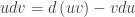 .
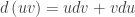
.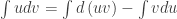 . By the FTC the first term on the right can be simplified giving the formula for Integration by Parts:
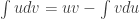
 in which there is a combination of functions that are usually of different types – here a polynomial and a trig function.
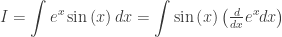
 . Here we make the substitutions
 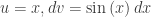 and from these we compute
  . (There is no need for the +C here; it will be included later). Making these substitutions gives

 and
and  the result is
