
 A reader recently asked me to do a post answering some questions about differential equations:
The 2016 AP Calculus course description now includes a new statement about domain restrictions for the solutions of differential equations. Specifically, EK 3.5A3 states “Solutions to differential equations may be subject to domain restrictions.” [The current 2020 CED uses the same wording in Essential Knowledge statement FUN-7.E.3] Could you write a blog post discussing (1) an example of how to determine the domain restriction; (2) speculating on whether one of the points for the differential equation on the free response will be allotted for specifying the restriction; and (3) speculating whether this concept could appear on the multiple choice and if so how.
First, let me compliment him on noticing EK 3.5A3. I overlooked it and have not seen anyone pick up on this yet. It seems to be a new item in the course description. Don’t panic. In the current 2020 CED EK FUN-7.E.3 says
A single question asking for the domain and range was asked before, but some time ago. Specifically, 2000 AB6 and 2006 AB 5 asked for the domain of the solution of a differential equation (see below for both). These are the only instances I can find that required students to find the domain of the solution.
Since 2008 many of the scoring standards included the domain, but they were not required to earn any points. These are discussed below. The domains were included in the solution, I suspect, because the standards are made public, and the readers want to publish the most complete answer.
What is required of the domain?
The generally accepted requirements are that the solution of a differential equation must be a function whose domain (1) must be an open interval, (2) on which the differential equation is true, and (3) contains the initial condition. Comments:
- The interval must be open since derivatives are not defined at the endpoints of intervals. The derivative is a two-sided limit and at an endpoint you can only approach from one side. While one-sided derivatives may be defined, they are a more burdensome requirement and not necessary.
- Practically speaking, this means that the solution may not cross a vertical asymptote or go through a point where the function is undefined; it must stay on the side where the initial condition is.
- The differential equation must be true in the sense that substituting the solution and its derivative(s) into the differential equation must result in an identity. (See 2007 AB 4(b) for practice).
- And of course, the initial condition point’s x-coordinate must be in the domain.
Teachers sometimes ask why we cannot just skip over an asymptote or an undefined point. When you do this, you are then working with a piecewise function. No problems there, but consider that on the piece(s) outside the domain as described above, you could have any function you want and still meet the three requirements above.
Finding the domain.
Here are some examples. Notice that the differential equation, its solution, and the initial condition all come into consideration.
2000 AB 6: After finding the solution 

![\displaystyle x>\sqrt[3]{\frac{-e}{2}}](https://s0.wp.com/latex.php?latex=%5Cdisplaystyle+x%3E%5Csqrt%5B3%5D%7B%5Cfrac%7B-e%7D%7B2%7D%7D&bg=ffffff&fg=333333&s=0&c=20201002)
2006 AB 5: Will be discussed below in answer to another question he asked.
2008 AB 5: The differential equation is undefined at x = 0 and the initial condition is to the right of this. So, the domain is all positive numbers.
2011 AB5/BC5: The domain is given in the stem; Time starts now and the differential equation applies “for the next 20 years”, so, 0 < x < 20
2013 AB 6: The solution is 

2013 BC 5: The solution, 
2014 AB 6: Neither the equation, nor the solution, 
2016 AB 4: The differential equation is 


2017 AB 4: The endpoints of the domain are stated in the stem of the problem. The time t begins when the potato is removed from the oven so t > 0 and the differential equation in (c) is given for t < 10. So the domain is 0 < t < 10.
2018 AB 6: Both the differential equation and its general solution are defined for all Real numbers:

All of these require no “calculus”- they are “find the domain” questions from pre-calculus with the concern about vertical asymptotes. There are some other considerations. A longer and far more detailed discussion of this can be found in “The Domain of Solutions to Differential Equations”, by former chief reader Larry Riddle.
I think that answers the first question my reader asked. As to his second and third questions, I guess the answer is yes. At some point students will be asked to state the domain of a differential equation. My guess is it will be a fairly easy one-point part of a free-response question. If solving the differential equation is necessary, then it seems too long for a multiple-choice question. This is all guesswork on my part; I have no knowledge of what’s on future exams.
2019 AB 4: The solution is a polynomial and there valid for all Real numbers.
2021 AB 6: The solution contains a power of e. The domain is all Real numbers.
2021 BC 4: The solution contains terms with ln(x). The domain is all x > 0.
2022 AB 5: The domain is all Real Numbers
My reader also asked about absolute value
Another question that may be related to this topic is the relevancy of the absolute value signs in the solutions to differential equations. When can they be kept in the solution, and when are they redundant?
Absolute values can really confuse kids. See my posts “Absolutely” and “Absolute Value.” Pre-calculus topics, yes, but they come back again and again.
Here are two examples about absolute values and domains:
2005 AB 6: After separating the variables and applying the initial condition we arrive at 


2006 AB 5. The initial value question is to solve 
After a few steps we arrive at 


The domain was asked for. Since it is given that 


I really appreciate questions from readers, so if you want to ask about some topic please ask me at lnmcmullin@aol.com . I’m always looking for new topics to write about – or said a different way, I’m running out of ideas!
.
Revised 4-3-18
Revised 12-23-2018 to include the 2017 and 2018 differential equation questions.
Revised 11-23-2020 – 2019 exam
Revised 1-11-2021
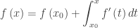 ,
, is the initial time, and
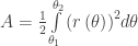
  is the initial amount. Since this is one of the main interpretations of the definite integral the concept may come up in a variety of situations.
 is the initial time, and
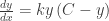
  , where k > 0 is the constant of proportionality, or by
 and
and 
 (D is the constant of integration formally known as “+C.”)
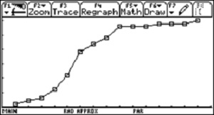
 indicate the location of a horizontal asymptote. There are horizontal asymptotes at y = 0 and y = C.
  , all the factors of the differential equation are positive. This indicates that the function is increasing. Near y = 0 and y = C one factor or the other is small, approaching 0: the graph of the solution (heavy blue line) is leveling off and approaching y = C from below as an asymptote. If the graph is extended into the second quadrant (thin blue line), it approaches the x-axis from above as an asymptote.
 the values of the slope (differential equation) remain positive but decrease indicating that the graph is now increasing and concave down. After this point the two factors of the differential equation switch values; that is, moving the same distance left and right of this point the product will be the same, but the values of each factor will have switched. Thus, the point where
  .
. with sliders for k and C.


 grams/cm where x is measured from one end of the rod. To find the total mass we think of cutting the rod in the very small pieces. (Think partition: each piece has a length of
  in which the density is nearly constant say
  . The limit of this expression as
  gives the total mass in grams:
 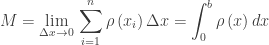 Notice that
  is the length of the rod. This is multiplied by the density to find the mass.
 people per square mile, where r is the distance from the center of the lake, in miles. Which of the following expressions gives the number of people who live within 1 mile of the lake?
 (B)
(B) 
 (D)
(D) 
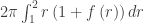
 where
where  is the distance from the center of the lake (this is the circumference of the ring), the width of this ring (rectangle) is
  . In this ring (rectangle) the population density is people per square mile, so the population in the ring is
  approximated by multiplying the area by the density:
  . Adding these gives a Riemann sum whose limit gives the total population:
 Answer (D).
 is the area of the city; this is multiplied by the population density to find the population.
 people per square mile. Which of the following expressions gives the population of the city?
 (B)
(B)  (C)
(C) 
 (E)
(E) 
 miles to the right of the river has an area of
  . The population in each such strip is found by multiplying the area by the density function; this gives
  . These are then added forming a Riemann sum, etc.
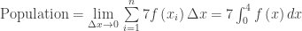 Answer (B)
 . Find the mass of a column of air 25 km high with a square base 3 meters on a side sitting on the surface of the earth.
 . The mass of this slice is
  . The sum of these slices gives a Riemann sum whose limit gives the total volume:

