One common question from students first learning about series is how to know which convergence test to use with a given series. The first answer is: practice, practice, practice. The second answer is that there is often more than one convergence test that can be used with a given series.
I will illustrate this point with a look at one series and the several tests that may be used to show it converges. This will serve as a review of some of the tests and how to use them. For a list of convergence tests that are required for the AP Calculus BC exam click here.
To be able to use these tests the students must know the hypotheses of each test and check that they are met for the series in question. On multiple-choice questions students do not need to how their work, but on free-response questions (such as checking the endpoints of the interval of convergence of a Taylor series) they should state them and say that the series meets them.
For our example we will look at the series 
Spoiler: Except for the first two tests to be considered, the other tests are far more work than is necessary for this series. The point is to show that several tests may be used for a given series, and to practice the other tests.
The Geometric Series Test is the obvious test to use here, since this is a geometric series. The common ratio is (–1/3) and since this is between –1 and 1 the series will converge.
The Alternating Series Test (the Leibniz Test) may be used as well. The series alternates signs, is decreasing in absolute value, and the limit of the nth term as n approaches infinity is 0, therefore the series converges.
The Ratio Test is used extensively with power series to find the radius of convergence, but it may be used to determine convergence as well. To use the test, we find
 Since the limit is less than 1, we conclude the series converges.
Absolute Convergence
A series,  , is absolutely convergent if, and only if, the series
  converges. In other words, if you make all the terms positive, and that series converges, then the original series also converges. If a series is absolutely convergent, then it is convergent. (A series that converges but is not absolutely convergent is said to be conditionally convergent.)
The advantage of going for absolute convergence is that we do not have to deal with the negative terms; this allows us to use other tests.
Applied to our example, if the series  converges, then our series
  will converge absolutely and converge.
The Geometric Series Test can be used again as above.
The Integral Test says if the improper integral  converges, then our original series will converge absolutely.
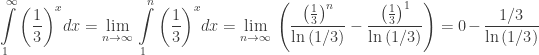
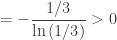 since ln(1/3) < 0.
The limit is finite, so our series converges absolutely, and therefore converges.
The Direct Comparison Test may also be used. We need to find a positive convergent series whose terms are term-by-term greater than the terms of our series. The geometric series  meets these two requirements. Therefore, the original series converges absolutely and converges.
The Limit Comparison Test is another possibility. Here we need a positive series that converges; we can use again. We look at
 and since the series in the denominator converges, our series converges absolutely.
So, for this example all the convergences that may be tested on the AP Calculus BC exam may be used with the single exception of the p-series Test which cannot be used with this series.
Teaching suggestions
- While the convergence of the series used here can be done all these ways, other series lend themselves to only one. Stress the form of the series that works with each test. For example, the Limit Comparison Test is most often used for rational expressions with the numerator of lower degree than the denominator and for expressions involving radicals of polynomials. The comparison is made with a p-series of whatever degree will make the numerator and denominator the same degree allowing the limit to be found.
- Most textbooks, after explaining each test and giving exercises on them, include a series of mixed exercises that require all the test covered up to that point. A good way to use this set is to assign students to state which test they would try first on each series. Discuss the opinions of the class and work any questions that students are unsure of or on which several ways are suggested.
- Give your students the series above, or a similar one, and have them prove its convergence using each of the convergence tests as was done above.
- Divide your class into groups and assign each group the series and one of the convergence tests. Ask them to use the test to prove convergence and then discuss the results as a group.
Of course, I didn’t really answer the question, did I? Check What Convergence Test Should I use Part 2
Updated February 23, 2013


 be a function that is positive, decreasing, and continuous for
  ; and let
  for
for 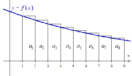
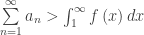 Assume that the improper integral
  diverges.
 . (NB: this series starts at n = 2.) Since
  to this gives the original series,
 θ
θ θ
θ to convert from polar to parametric form,
 and
and  (Hint: use the product rule on the equations in the previous bullet).
 (motion towards or away from the pole),
  (motion in the vertical direction) or
  .
. is a necessary condition for convergence. It is not sufficient; if the limit is zero then the series may converge. Look for a convergence test.
 converges if
  and diverges if
  . A p-series is often a good test to use for comparison in the next two tests. However, any series whose convergence you are sure of may be used.
 would be a geometric series except for the radical. Compare it with the geometric series
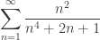 can be compared with the p-series
  . The hint here is that ignoring the lower power terms in the denominator and reducing we see that the original series looks like
  while similar, has terms greater than the terms of
  are larger than the harmonic series
  a divergent p-series, so this series diverges.
 Series with radicals also are candidates for the limit comparison test. Since the general terms is approximately
  Compare this with
  or
or  are candidates for the Ratio Test. Both Converge.
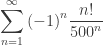 appears to be a candidate for the alternating series test. However, for large values of n > 530 the terms increase in absolute vale, so the alternating series test cannot be applied. The ratio test works here, but since the terms do not approach 0 as n increases, the nth-term test for divergence also works. This series diverges.
 or the equivalent vector
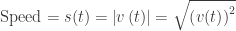
  . The path is the curve traced by the parametric equations or the tips of the position vector. .
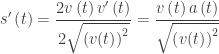
 . The vector sum of the components gives the direction of motion. Attached to the tip of the position vector this vector is tangent to the path pointing in the direction of motion.
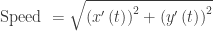 . (Notice that this is the same as the speed of a particle moving on the number line with one less parameter: On the number line
  .)
.) .
. , or even
  form. The pointed brackets seem to be the most popular right now, but all common notations are allowed and will be recognized by readers.
 . Notice that this is the integral of the speed (rate times time = distance).
 . See
. See 