July | 2017 | Teaching Calculus

Cubic Symmetry

Some things are fairly obvious. For example, if you look at the graphs of a few cubic equations, you might think that each is symmetric to a point and on closer inspection the point of symmetry is the point of inflection.

This is true and easy to prove. You can find the point of inflection, and then show that any point a certain distance horizontally on one side is the same distance above (or below) the point of inflection as a point the same distance horizontally on the other side is below (or above). Another way is to translate the cubic so that the point of inflection is at the origin and then show the resulting function is an odd function (i.e. symmetric to the origin).

But some other properties are not at all obvious. How someone thought to look for them is not even clear.

Tangent Line.

If you have cubic function with real roots of x = a, x = b, and x = c not necessarily distinct, if you draw a tangent line at a point where x is the average of any two roots, x = ½(a + b), , then this tangent line intersects the cubic on the x-axis at exactly the third root, x = c. Here is a Desmos graph illustrating this idea.

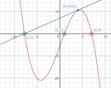
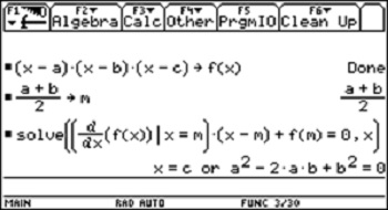
Here is a proof done with a CAS. The first line is a cubic expressed in terms of its roots. The third line asks where the tangent line at x = m intersects the x-axis. The last line is the answer: x = c or whenever a = b (i.e. when the two roots are the same, in which case the tangent line is the x-axis and of course also contains x = c.

Areas
Even harder to believe is this: Draw a tangent line anywhere on a cubic. This tangent will intersect the cubic at a second point and the line and the cubic will define a region whose area is A1. From the second point draw a tangent what intersects the cubic at a third point and defines a region whose area is A2. The ratio of the areas A2/A1 = 16. I have no idea why this should be so, but it is.

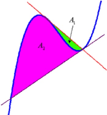
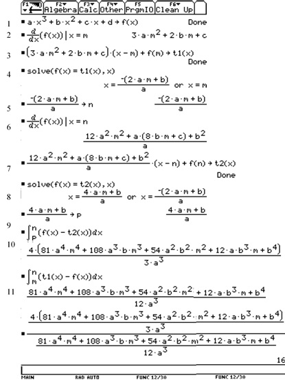
Here is a proof, again by CAS: The last line marked with a square bullet is the computation of the ratio and the answer, 16, is in the lower right,

And if that’s not strange enough, inserting two vertical lines defines other regions whose areas are in the ratios shown in the figure below.

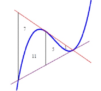
Who’d a thunk it?

Today, for some summer fun, let’s look at synthetic division a/k/a synthetic substitution. I’ll assume you all know how to do that since it is a pretty common pre-calculus topic and even comes up again in calculus.

Why Does Synthetic Division Work?

An example: consider the polynomial

$P(x)=2{{x}^{4}}-3{{x}^{3}}-11{{x}^{2}}+14x-1$ .

This can be written in nested form like this

$P(x)=((((2x-3)x-11)x+14)x-1)$

To evaluate this last expression at, say x = 2, we do the arithmetic as follows:

2 x 2 – 3 = 1
2 x 1 – 11 = –9
2 x (–9) + 14 = –4
2 x (–4) – 1 = – 9 = f(2)

Notice that this requires only multiplication and addition or subtraction, no raising to powers. More to the point, this is the same arithmetic, in the same order when you do the evaluation by synthetic division, and the work is a little easier to keep track of.

$\begin{matrix} {} & 2 & -3 & -11 & 14 & -1 \\ 2) & 2 & 1 & -9 & -4 & -9 \\ \end{matrix}\begin{matrix} {} \\ \,=P(2) \\ \end{matrix}$

Synthetic division has another advantage: the other numbers in the second row are the coefficients of a quotient polynomial, a polynomial of one less degree that the original. So,

$\displaystyle \frac{P(x)}{x-2}=2{{x}^{3}}+{{x}^{2}}-9x-4+\frac{-9}{x-2}$

The Remainder Theorem and the Factor Theorem

In general, a polynomial of degree n, divided by a linear factor (x – a) gives a polynomial Q(x) of degree n – 1 and a remainder R

$\displaystyle \frac{P(x)}{x-a}=Q(x)+\frac{R}{x-a}$

$P(x)=Q(x)(x-a)+R$

From here it is easy to see that $P(a)=R$ . This is called the remainder theorem. It has a corollary called the factor theorem: If R = 0, then (x – a) is a factor of P(x).

Calculus

But wait there is more: differentiating the equation above using the product rule gives

${P}'(x)=Q(x)(1)+Q(x)(x-a)+0$ and substituting x = a gives

${P}'(a)=Q(a)$ . The value of the quotient polynomial at a is the derivative of the original polynomial at a.

Of course, we could also rewrite the same equation as $\displaystyle \frac{P(x)-P(a)}{x-a}=Q(x)$ . Then

$\displaystyle {P}'(a)=\underset{x\to a}{\mathop{\lim }}\,\frac{P(x)-P(a)}{x-a}=\underset{x\to a}{\mathop{\lim }}\,Q(x)=Q(a)$

Taylor Series

But wait, there’s even more.

A polynomial is a Maclaurin series in which all the terms after the n^th term are zero. When you students are first learning how to write a Taylor series, by finding all the derivatives and substituting in the general term, a good exercise is to have them write the Taylor series for a polynomial centered away from the origin. For the example above:

$P(x)=-9-2\left( x-2 \right)+19{{\left( x-2 \right)}^{2}}+13{{\left( x-2 \right)}^{3}}+2{{\left( x-2 \right)}^{4}}$

Then ask them to expand the expression above and collect term etc. They should get the original polynomial again (and have some great practice expand powers of a binomial).

Can synthetic division help us? Yes, of course. Here, is the original computation again:

$\begin{matrix} {} & 2 & -3 & -11 & 14 & -1 \\ 2) & 2 & 1 & -9 & -4 & -9 \\ \end{matrix}\begin{matrix} {} \\ \,=P(2) \\ \end{matrix}$

If we ignore the –9 and divide the quotient numbers by 2 we get

$\begin{matrix} {} & 2 & 1 & -9 & -4 \\ 2) & 2 & 5 & 1 & -2 \\ \end{matrix}\begin{matrix} {} \\ \ ={P}'(2) \\ \end{matrix}$

$\begin{matrix} {} & 2 & 5 & 1 \\ 2) & 2 & 9 & 19 \\ \end{matrix}\begin{matrix} {} \\ \ =\frac{{{P}'}'(2)}{2} \\ \end{matrix}$

And again

$\begin{matrix} {} & 2 & 9 \\ 2) & 2 & 13 \\ \end{matrix}\begin{matrix} {} \\ \ =\frac{{{{P}'}'}'\left( 2 \right)}{3!} \\ \end{matrix}$

One more time

$\begin{matrix} {} & 2 \\ 2) & 2 \\ \end{matrix}\begin{matrix} {} \\ \ =\frac{{{P}^{(4)}}\left( 2 \right)}{4!} \\ \end{matrix}$

What do you see? Right, the last numbers in each computation, –9, –2, 19, 13, and 2, are the coefficients of the Taylor polynomial!

If you really want to dive this home and have some more summer fun here’s the start of a proof (at least for n = 4). Let

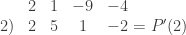
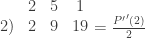
$P(x)={{c}_{4}}{{x}^{4}}+{{c}_{3}}{{x}^{3}}+{{c}_{2}}{{x}^{3}}+{{c}_{1}}x+{{c}_{0}}$ and divide this by a:

$\begin{matrix} {} & {{c}_{4}} & {{c}_{3}} & {{c}_{2}} & {{c}_{1}} & {{c}_{0}} \\ a) & {{c}_{4}} & {{c}_{4}}a+{{c}_{3}} & {{c}_{4}}{{a}^{2}}{{+}_{{}}}{{c}_{3}}a+{{c}_{2}} & {{c}_{4}}{{a}^{3}}+{{c}_{3}}{{a}^{2}}+{{c}_{a}}a+{{c}_{1}} & {{c}_{4}}{{a}^{4}}+{{c}_{3}}{{a}^{3}}+{{c}_{a}}{{a}^{2}}+{{c}_{1}}a+{{c}_{0}}=P(a) \\ \end{matrix}$

Again

$\begin{matrix} {} & {{c}_{4}} & {{c}_{4}}a+{{c}_{3}} & {{c}_{4}}{{a}^{2}}{{+}_{{}}}{{c}_{3}}a+{{c}_{2}} & {{c}_{4}}{{a}^{3}}+{{c}_{3}}{{a}^{2}}+{{c}_{2}}a+{{c}_{1}} \\ a) & {{c}_{4}} & 2{{c}_{4}}a+{{c}_{3}} & 3{{c}_{4}}{{a}^{2}}+2{{c}_{3}}a+{{c}_{2}} & 4{{c}_{4}}{{a}^{3}}+3{{c}_{3}}{{a}^{2}}+2{{c}_{2}}a+{{c}_{1}} \\ \end{matrix}\begin{matrix} {} \\ \ ={P}'(a) \\ \end{matrix}$