Introducing Power Series 3

In my two posts immediately preceding this one I suggested an approach to introducing power series by kind of sneaking up on them starting with the tangent line (local linear) approximation and then going for a second-, third- and higher-degree polynomial that had the same value and same derivative values as the function at a point. These polynomials are called Taylor Approximating Polynomials centered at xa.  If a = 0 then they are called Maclaurin polynomials.

Next, we looked at the graphs of two of these one for ln(x) and one for sin(x). If you tried some others, I suggest you be sure to look at their graphs. We saw that the graphs of the polynomials “hugged” the original function and the higher the degree the closer they came to the function. But there was a difference: the ln(x) polynomials were close only in an interval about two units wide with xa in the center, while the polynomials for sin(x) seemed to be close to sin(x) over wider and wider intervals.

This brought several questions to mind. Hopefully, you can draw these and other questions out of your class and then discuss them as a preview of coming ideas and motivation to learn more . Here are the questions.

1. If there were an infinite number of terms, would the polynomial (now more properly called an infinite series) be the same as the function? Equal, that is. We are of course used to thinking in terms of limits by now. For some functions, such as the sin(x), it appears that this might be the case. But for others, such as ln(x), certainly not.  

2. How do you add an infinite number of terms? Good question to which I don’t have a ready answer. In cases like the sin(x) it looks like the sum would be sin(x). 

3. Over what interval is the approximation “good”? How do you find the interval? We need a way to find this interval, called the interval of convergence. The interval, as it turns out, can usually be found using the Ratio Test or some other means, For example, if the polynomial turns out to be a geometric series, then the interval depends on the common ratio of the series.  Is the interval the same for all functions? No; look at the two examples we have been working with.

4. How good is the approximation? A question you should ask with any approximation. There are several ways of determining this. The two primary ones are the Alternating Series Error Bound and the Lagrange Error Bound. I will discuss error bounds in a later post. 

5. Is there an easier way to build the polynomial? Do you have to figure out and evaluate all of the derivatives? Luckily, no. There are easier ways to find a number of series and that too will be the subject of a later post. But not all series; occasionally you will need to find the derivatives and do all the computations. So some practice with that is in order.

6. So okay, this is a lot of fun, but why bother? Polynomials are really easy to handle. They are easy to evaluate, differentiate and integrate. Other functions, not so much. We all learned that \sin \left( \tfrac{\pi }{6} \right)=\tfrac{1}{2} and values for other “special angles”, but what is sin(0.2)? Of course you usually find such information on a calculator: sin(0.2) = 0.198669331, but you can also find it with a few terms of the series for sin(x):

\sin (0.2)\approx 0.2-\frac{{{0.2}^{3}}}{3!}+\frac{{{0.2}^{5}}}{5!}=0.198669333

Notice that using only three terms you have an answer correct to 8 decimal places. So one answer is that  you can use the approximating polynomials to, wait for it, approximate. But there are other uses as well. Stay tuned.

Inrtoducing Power Series 2

In our last post we found that we could produce better and better polynomial approximations to a function. That is, we produced a set of polynomials of increasing degree that had the same value for the functions and its derivatives at a given point. To see what is going on I suggest we graph these approximating polynomials along with the given function.

We found that the polynomials \left( x-1 \right), \left( x-1 \right)+\left( -\tfrac{1}{2} \right){{\left( x-1 \right)}^{2}}, \left( x-1 \right)+\left( -\tfrac{1}{2} \right){{\left( x-1 \right)}^{2}}+\left( \tfrac{1}{6} \right){{\left( x-1 \right)}^{3}}, and \left( x-1 \right)+\left( -\tfrac{1}{2} \right){{\left( x-1 \right)}^{2}}+\left( \tfrac{1}{6} \right){{\left( x-1 \right)}^{3}}+\left( -\tfrac{1}{4!} \right){{\left( x-1 \right)}^{4}} produced approximations to the natural logarithm function at the point (1, 0). To see how this works, graph each of these polynomials, one after the other. See the figure below.

This slideshow requires JavaScript.

Notice that each polynomial comes closer to the graph of the graph of y = ln(x), the black graph, in the figures.

You students can do this on their graphing calculators or with a graphing program. More on how to do  this below.

Now do the same thing with the polynomials found for the sine function.

This slideshow requires JavaScript.

However, there is a difference. The sine polynomials seem to hug the sine graph over increasingly wider intervals while the logarithm polynomials do not. This may not be a surprise since the logarithm function has no values for x\le 0 while the polynomials do. The polynomials cannot come close to the graph if there is no graph.

Students should notice these things:

  • Successively higher degree polynomials seem to come closer to the graph of the function than the previous one.
  • The polynomials may exist outside the domain of the function (outside of x>0 for ln(x) for example).
  • The interval where the graphs are near the function is limited.

Taken together these two examples suggest several questions (which you can perhaps draw out of your class):

  1. If there were an infinite number of terms would the Polynomial be the same as the function?
  2. How do you add an infinite number of terms?
  3. Over what interval is the approximation “good”? Is the interval the same for all functions? How do you find the interval?
  4. How good is the approximation?
  5. Is there an easier way to build the polynomial? Do you have to figure out and evaluate all of the derivatives?

These questions will be the topic of my next post.

________________________________________

How to Graph these Polynomials using Winplot

You can enter each polynomial separately of course, but here is an easier way.

  1. After setting your viewing window (CTRL+V), push [F1] to get the explicit equation entry window and enter sin(x) (or the function you are interested in) and click [OK] to graph y = sin(x).
  2. Then push [F1] again and enter Sum( (-1)^(n+1)x^(2n-1)/(2n-1)! ,n,1,A) and click [OK]. The underlined part may be changed to the general term of any series.  The n identifies the variable, the 1 is the starting value of n and the A will be the final value which we will change.
  3. Next click on [ANIM] > [Individual] > [A]. This will bring up a slider. Enter 100 in the box and click [Set R] and then enter 0 and click [Set L]. This will make the A values change by exactly 1 allowing you to look at A = 1, 2, 3, 4, … in order.
  4. Click the tab on the “A” slider window box and see the various approximating polynomials “hug” the graph


Introducing Power Series 1

The next few posts will discuss a way to introduce Taylor and Maclaurin series to students. We will kind of sneak up on the idea without mentioning where we are going or using any special terms. In this post we will find a way of approximating a function with a polynomial of any degree we choose. In the next post we will look at the graph of these polynomials and finally suggest some questions for further thought.

Making Better Approximations

Students already know and have been working with the tangent line approximation of a function at a point (a, f(a)):

f(x)\approx f\left( a \right)+{f}'\left( a \right)\left( x-a \right)

ln(x):

For the function f\left( x \right)=\ln \left( x \right) 
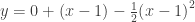
at the point (1, 0) ask your students to write the tangent line approximation: y=0+(1)(x-1) .Point out that this line has the same value as  ln(xand its derivative as at (1, 0).

Then suggest that maybe having a polynomial that has the same value, first derivative and second derivative might be a better approximation. Suggest they start with y=a+b\left( x-1 \right)+c{{\left( x-1 \right)}^{2}} and see if they can find values of a, b and c that will make this happen.

Since f\left( 1 \right)=0,{f}'\left( 1 \right)=1\text{ and }{{f}'}'\left( x \right)=-1 we can write

y=a+b\left( x-1 \right)+c{{\left( x-1 \right)}^{2}};\quad y\left( 1 \right)=a+0+0=0;\quad a=0

{y}'=b+2c\left( x-1 \right);\quad {y}'\left( 1 \right)=b+0=\tfrac{1}{1};\quad b=1

{{y}'}'=2c;\quad {{y}'}'\left( 1 \right)=c=-\tfrac{1}{{{1}^{2}}}=-1;\quad c=-\tfrac{1}{2}

y=0+\left( x-1 \right)-\tfrac{1}{2}{{\left( x-1 \right)}^{2}}

Then suggest they try a third degree polynomial starting with y=a+b\left( x-1 \right)+c{{\left( x-1 \right)}^{2}}+d{{\left( x-1 \right)}^{3}}
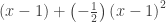
. Proceeding as above, all the numbers come out the same and we find that

\ln \left( x \right)\approx 0+\left( x-1 \right)+\left( -\tfrac{1}{2} \right){{\left( x-1 \right)}^{2}}+\left( \tfrac{1}{3} \right){{\left( x-1 \right)}^{3}}

Then go for a fourth- and fifth-degree polynomial until they discover the patterns. (The signs alternate, and the denominators are the factorial of the exponent.)

See if the class can write a general polynomial of degree N :

 \displaystyle \ln \left( x \right)\approx \sum\limits_{k=1}^{N}{\frac{{{\left( -1 \right)}^{k+1}}}{k}{{\left( x-1 \right)}^{k}}}

sin(x):

Then have the class repeat all this for a new function such as f\left( x \right)=\sin \left( x \right) 
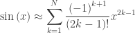
at the point (0, 0). This could be assigned as homework or group work. Ask them to do enough terms until they see the pattern. There will be patterns similar to ln(x ) and every other term (the even powers) will have a coefficient of zero.

\sin \left( x \right)\approx x-\tfrac{1}{3!}{{x}^{3}}+\tfrac{1}{5!}{{x}^{5}}-\tfrac{1}{7!}{{x}^{7}}+\tfrac{1}{9!}{{x}^{9}}

or in general the polynomial of degree N is

\displaystyle \sin \left( x \right)\approx \sum\limits_{k=1}^{N}{\frac{{{\left( -1 \right)}^{k+1}}}{\left( 2k-1 \right)!}{{x}^{2k-1}}}

How good is this approximation? Using only the first three terms of the polynomial above you will tell you that. Pretty close: correct to 5 decimal places.  Using four terms gives correct to 7 decimal places when rounded.

Finally, see if they can generalize this idea to any function f at any point on the function \left( {{x}_{0}},f\left( {{x}_{0}} \right) \right). This time you will not have the various derivatives as numbers, rather they will be expressions like . Work through the powers one at a time to go from y=a+b\left( x-{{x}_{0}} \right)+c{{\left( x-{{x}_{0}} \right)}^{2}}+d{{\left( x-{{x}_{0}} \right)}^{3}}+e{{\left( x-{{x}_{0}} \right)}^{4}}

and so on, until you get to

f\left( x \right)\approx f\left( {{x}_{0}} \right)+\frac{{f}'\left( {{x}_{0}} \right)}{1!}\left( x-{{x}_{0}} \right)+\frac{{{f}'}'\left( {{x}_{0}} \right)}{2!}{{\left( x-{{x}_{0}} \right)}^{2}}

\quad \quad \quad \quad \quad \quad \quad \quad \quad \quad \quad \quad \quad +\cdots +\frac{{{f}^{\left( N \right)}}\left( {{x}_{0}} \right)}{N!}{{\left( x-{{x}_{0}} \right)}^{N}}

For example the third derivative computation would look like this:

{{{y}'}'}'=3\cdot 2\cdot 1d+4\cdot 3\cdot 2e\left( x-{{x}_{0}} \right)

{{{y}'}'}'\left( {{x}_{0}} \right)=3\cdot 2\cdot 1d+4\cdot 3\cdot 2e(0)={{{f}'}'}'\left( {{x}_{0}} \right)

d=\frac{{{{f}'}'}'\left( {{x}_{0}} \right)}{3!}

The computations here are perhaps a little different than what students have seen, so take your time doing this. Two or even three class days may be necessary.

Notice these things:

  • The first two terms are the tangent line approximation.
  • The various derivatives are numbers that must be calculated.
  • All the terms of any degree are the same as the terms of the previous degree with one additional term.

Next post in this series: Looking at all this graphically.

(Typos in an earlier version of this post have been corrected – LMc)