Unit 3 – Differentiation: Composite, Implicit, and Inverse Function

Posted on September 21, 2021 by Lin McMullin

Unit 3 covers the Chain Rule, differentiation techniques that follow from it, and higher order derivatives. (CED – 2019 p. 67 – 77). These topics account for about 9 – 13% of questions on the AB exam and 4 – 7% of the BC questions.

Topics 3.1 – 3.6

Topic 3.1 The Chain Rule. Students learn how to apply the Chain Rule in basic situations.

Topic 3.2 Implicit Differentiation. The Chain Rule is used to find the derivative of implicit relations.

Topic 3.3 Differentiation Inverse Functions. The Chain Rule is used to differentiate inverse functions.

Topic 3.4 Differentiating Inverse Trigonometric Functions. Continuing the previous section, the ideas of the derivative of the inverse are applied to the inverse trigonometric functions.

Topic 3.5 Selecting Procedures for Calculating Derivatives. Students need to be able to choose which differentiation procedure should be used for any function they are given. This is where you can review (spiral) techniques from Unit 2 and practice those from this unit.

Topic 3.6 Calculating Higher Order Derivatives. Second and higher order derivatives are considered. Also, the notations for higher order derivatives are included here.

Topics 3.2, 3.4, and 3.5 will require more than one class period. You may want to do topic 3.6 before 3.5 and use 3.5 to practice all the differentiated techniques learned so far. The suggested number of 40 – 50-minute class periods is about 10 – 11 for AB and 8 – 9 for BC. This includes time for testing etc.

Posts on these topics include:

Foreshadowing the Chain Rule

The Power Rule Implies Chain Rule

The Chain Rule

Seeing the Chain Rule

Derivative Practice – Numbers

Derivative Practice – Graphs

Experimenting with CAS – Chain Rule

Implicit Differentiation of Parametric Equations

Adapting 2021 AB 5

This series of posts reviews and expands what students know from pre-calculus about inverses. This leads to finding the derivative of exponential functions, a^x, and the definition of e, from which comes the definition of the natural logarithm.

Inverses Graphically and Numerically

The Range of the Inverse

The Calculus of Inverses

The Derivatives of Exponential Functions and the Definition of e and This pair of posts shows how to find the derivative of an exponential function, how and why e is chosen to help this differentiation.

Logarithms Inverses are used to define the natural logarithm function as the inverse of e^x. This follow naturally from the work on inverses. However, integration is involved and this is best saved until later. I will mention it then.

Here are links to the full list of posts discussing the ten units in the 2019 Course and Exam Description.

Limits and Continuity – Unit 1 (8-11-2020)

Definition of t he Derivative – Unit 2 (8-25-2020)

Differentiation: Composite, Implicit, and Inverse Function – Unit 3 (9-8-2020) THIS POST

LAST YEAR’S POSTS – These will be updated in coming weeks

2019 CED – Unit 4 Contextual Applications of the Derivative Consider teaching Unit 5 before Unit 4

2019 – CED Unit 5 Analytical Applications of Differentiation Consider teaching Unit 5 before Unit 4

2019 – CED Unit 6 Integration and Accumulation of Change

2019 – CED Unit 7 Differential Equations Consider teaching after Unit 8

2019 – CED Unit 8 Applications of Integration Consider teaching after Unit 6, before Unit 7

2019 – CED Unit 9 Parametric Equations, Polar Coordinates, and Vector-Values Functions

2019 CED Unit 10 Infinite Sequences and Series

Differentiation: Composite, Implicit, and Inverse Function – Unit 3

Posted on September 8, 2020 by Lin McMullin

This is a re-post and update of the third in a series of posts from last year. It contains links to posts on this blog about the differentiation of composite, implicit, and inverse functions for your reference in planning. Other updated posts on the 2019 CED will come throughout the year, hopefully, a few weeks before you get to the topic. Unit 3 covers the Chain Rule, differentiation techniques that follow from it, and higher order derivatives. (CED – 2019 p. 67 – 77). These topics account for about 9 – 13% of questions on the AB exam and 4 – 7% of the BC questions.

Topics 3.1 – 3.6

Topic 3.1 The Chain Rule. Students learn how to apply the Chain Rule in basic situations.

Topic 3.2 Implicit Differentiation. The Chain Rule is used to find the derivative of implicit relations.

Topic 3.3 Differentiation Inverse Functions. The Chain Rule is used to differentiate inverse functions.

Topic 3.4 Differentiating Inverse Trigonometric Functions. Continuing the previous section, the ideas of the derivative of the inverse are applied to the inverse trigonometric functions.

Topic 3.6 Calculating Higher Order Derivatives. Second and higher order derivatives are considered. Also, the notations for higher order derivatives are included here.

Posts on these topics include:

Foreshadowing the Chain Rule

The Power Rule Implies Chain Rule

The Chain Rule

Seeing the Chain Rule

Derivative Practice – Numbers

Derivative Practice – Graphs

Experimenting with CAS – Chain Rule

Implicit Differentiation of Parametric Equations

Inverses Graphically and Numerically

The Range of the Inverse

The Calculus of Inverses

Logarithms Inverses are used to define the natural logarithm function as the inverse of e^x. This follows naturally from the work on inverses. However, integration is involved, and this is best saved until later. I will mention it then.

Here are links to the full list of posts discussing the ten units in the 2019 Course and Exam Description.

Limits and Continuity – Unit 1 (8-11-2020)

Definition of the Derivative – Unit 2 (8-25-2020)

Differentiation: Composite, Implicit, and Inverse Function – Unit 3 (9-8-2020) THIS POST

LAST YEAR’S POSTS – These will be updated in the coming weeks

2019 CED – Unit 4 Contextual Applications of the Derivative Consider teaching Unit 5 before Unit 4

2019 – CED Unit 5 Analytical Applications of Differentiation Consider teaching Unit 5 before Unit 4

2019 – CED Unit 6 Integration and Accumulation of Change

2019 – CED Unit 7 Differential Equations Consider teaching after Unit 8

2019 – CED Unit 8 Applications of Integration Consider teaching after Unit 6, before Unit 7

2019 – CED Unit 9 Parametric Equations, Polar Coordinates, and Vector-Values Functions

2019 CED Unit 10 Infinite Sequences and Series

Limit of Composite Functions

Posted on August 26, 2019 by Lin McMullin

Recently, a number of questions about the limit of composite functions have been discussed on the AP Calculus Community bulletin board and also on the AP Calc TEACHERS – AB/BC Facebook page. The theorem that we would like to apply in these cases is this:

If f is continuous at b and $\underset{{x\to a}}{\mathop{{\lim }}}\,g\left( x \right)=b$ , then $\underset{{x\to a}}{\mathop{{\lim }}}\,f\left( {g\left( x \right)} \right)=f\left( b \right)$ .

That is, $\underset{{x\to a}}{\mathop{{\lim }}}\,f\left( {g\left( x \right)} \right)=f\left( {\underset{{x\to a}}{\mathop{{\lim }}}\,g\left( x \right)} \right)$

The problem is that in the examples one or the other of the hypotheses (continuity or the existence of $\underset{{x\to a}}{\mathop{{\lim }}}\,g\left( x \right)$ ) is not met. Therefore, the theorem cannot be used. This does not mean that the limits necessarily do not exist, rather that we need to find some other way of determining them. We need a workaround. Let’s look at some.

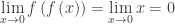
Example 1: The first example is from the 2016 BC International exam, question 88. Students were given the graph at the right and asked to find $\displaystyle \underset{{x\to 0}}{\mathop{{\lim }}}\,f\left( {1-{{x}^{2}}} \right)$ .

At first glance it appears that as x approaches zero, $\left( {1-{{x}^{2}}} \right)$ approaches 1 and the limit does not exist since f is not continuous at 1, so the theorem cannot be used. However, on closer examination, we see that $\left( {1-{{x}^{2}}} \right)$ is always less than 1, so $\left( {1-{{x}^{2}}} \right)$ is approaching 1 from the left (or from below). Therefore, as f approaches 1 from the left $\displaystyle \underset{{x\to 0}}{\mathop{{\lim }}}\,f\left( {1-{{x}^{2}}} \right)=\underset{{x\to {{1}^{-}}}}{\mathop{{\lim }}}\,f\left( x \right)=3$

Another approach is to try to write the equation of f. Although we cannot be certain, it appears that: $f\left( x \right)={{x}^{2}}+2,x<1$ .

Then, $f\left( {1-{{x}^{2}}} \right)={{\left( {1-{{x}^{2}}} \right)}^{2}}+2={{x}^{4}}-2{{x}^{2}}+3,x<1$ . In this form the limit is obviously 3.

Example 2: The second example is also based on a graph. Given the graph of a function f, shown at the left, what is $\displaystyle \underset{{x\to 0}}{\mathop{{\lim }}}\,f\left( {f\left( x \right)} \right)$ ?

$\underset{{x\to 0}}{\mathop{{\lim }}}\,f\left( x \right)=2$ . Since f is not continuous at 2, the theorem cannot be used. But, notice that as x approaches 0 from both sides, the limit 2 is approached from the left (from below). So we need to find the value of f as its argument approaches ${{2}^{-}}$ . From the graph, this value is zero; So, $\underset{{x\to 0}}{\mathop{{\lim }}}\,f\left( {f\left( x \right)} \right)=0$

To clarify this a little more, let’s look at a similar problem suggested by Sondra Edwards on the Facebook site: Consider this similar function:

Now as we approach 0 from both sides $\underset{{x\to 0}}{\mathop{{\lim }}}\,f\left( x \right)=2$ approached from both sides. But now f(2) does not exist (DNE). (This is the “outside” f, which is not continuous here.) This time, the limiting value, 2, is approached from both sides. Therefore, $\underset{{x\to 0}}{\mathop{{\lim }}}\,f\left( {f\left( x \right)} \right)$ DNE. There is no way to work around the discontinuity.

For a similar question see here

Example 3: If $\displaystyle f\left( x \right)=\frac{1}{x},x\ne 0$ , what is $\displaystyle \underset{{x\to 0}}{\mathop{{\lim }}}\,f\left( {f\left( {x)} \right)} \right)$ ?

Here again, the theorem cannot be used, since the “inside” function has no limit as x approaches 0. But, this function is its own inverse, so $\displaystyle f\left( {f\left( {x)} \right)} \right)=x$ , and $\displaystyle \underset{{x\to 0}}{\mathop{{\lim }}}\,f\left( {f\left( x \right)} \right)=\underset{{x\to 0}}{\mathop{{\lim }}}\,x=0$