AP Exam Review 2024

For several years now, I’ve been posting a series of notes on reviewing for the AP Calculus Exams. The questions on the AP Calculus exams, both multiple-choice and free response, fall into ten types. I’ve published posts on each. The ten types have not changed over the years, so there is not much to add. They are updated from time to time. The posts may be found under the “Blog Guide” tab above: click on AP Exam Review. The same links are below with a brief explanation of each.

This year’s AP Calculus exams will be given on Monday May 13, 2024, at 8:00 am local time.

I hope these will help as you, teachers and students, to review for this year’s exam.

General information and suggestions for teachers

  • AP Exam Review – Suggestions, hints, information, and other resources for reviewing. How to get started. What to tell your students. Simulated (mock) exams.
  • To dx or not to dx – Yes, use past exams and the scoring guideline to review, but don’t worry about the fine points of scoring; be more stringent than the readers.
  • Practice Exams – A Modest Proposal Like it or not (and the AP folks certainly do not) the answers are all online. What to do about that. Don’t overlook the replies at the end of this post.

General Information for students

Why Review? To make mistakes!

How, not only to survive, but to Prevail… Things students should know to do well on the exams. Copy this article for your students or share the link with them.

The Ten Type Questions.

Other than simply finding a limit, a derivative, an antiderivative, or evaluating a definite integral, the AP Calculus exam questions fall into these ten types. These are different from the ten units in the CED. Students are often expected to use knowledge from more than one AP Calculus unit in a single question.

These posts outline what each type of question covers and what students should be able to do. They include references to good questions, free-response and multiple-choice, and links to other posts on the topic.

These ten types appear in multiple-choice and free response questions. This type analysis provides an index to the questions by type. In addition the multiple-choice questions include straightforward questions (find a limit, compute a derivative, etc.)

Type 1 questions – Rate and accumulation questions. Contextual questions about things that are changing. Careful reading is the first step. Good graphing calculator skills are essential since this is usually a calculator active question.

  • Type 3 questions – Graph analysis. Given the derivative often as a graph, students must answer questions about the function – extreme values, increasing, decreasing, concavity, etc.
  • Type 4 questions – Area and volume problems. Student must find the area of a region enclosed by one or more curves, find the volume of a solid with regular cross-sections, and/or find the volume of a solid of revolution (which is, of course, a regular cross-section).
  • Type 6 questions – Differential equations. Students are asked to solve a first-order separable differential equation, work with a slope field, or other related ideas. BC students may be asked to use Euler’s Method to approximate a value and discuss the logistic equation.
  • Type 7 questions – Miscellaneous. These include finding the first and second derivative of implicitly defined relation, solving a related rate problem or other topics not included in the other types.
  • Type 10 questions – Sequences and Series (BC topic) Questions ask student to determine the convergence of series using various convergence tests and to write and work with a Taylor and Maclaurin series, find its radius and interval of convergence.

The notes always available from the menu line at the top of the page: click on Blog Guide > AP Exam Review


Also, Calc-Medic has posted a searchable database of all the AP Calculus Free-response questions from 1998 on. The link is here. While you’re there take a look at their website which has lots of resources and free lesson plans. For more on Calc-medic see this post.


Updates: March 9, 2023 – Calc-medic, March 2, 2024

Why Review?

The reason you review is TO MAKE MISTAKES!

When you’re reviewing for the AP Calculus exams your goal is to make mistakes. Why make mistakes? Easy: to find out what you’re doing wrong so you can fix it. And to find out what you don’t know so you can learn it.  

Your teacher will assign free-response questions, FRQs, from real AP Calculus exams from past years. Give yourself about 15 minutes and try to answer the question. (Fifteen minutes is about the time you have for each FRQ on the exam.) After fifteen minutes, stop. Check your work.

The questions, answers, solutions, and most importantly the scoring guidelines for FRQs are all online here for AB, and here for BC. Each FRQ is worth nine points. The scoring guidelines will show you what must be on your paper to earn each point.

Now you can copy the absolutely perfect answer for your FRQs and hand it in to your teacher. This won’t impress or fool your teacher because he or she has the guidelines too. More importantly this won’t help you. When reviewing mistakes are good. Study your mistakes and learn from them.

  • If you made a simple arithmetic or algebra mistake, learn to be more careful. One very common mistake is simplifying your answer incorrectly. Remember, you do not have to simplify numerical or algebraic answers. If you write “ 1 + 1 “ and the correct answer is 2, the “ 1 + 1 ” earns the point. But if you simplified it to 3, you lose the point you already earned. (The standards show simplified answers, so the readers will know what they are for (foolish?) students who chose to simplify.) simplifying also wastes time.
  • If you’re unsure how to write justifications, explanations, and other written answers, use the scoring guidelines as samples or templates. Learn to say what you need to say. Don’t say too much. You will not earn full credit for the correct answer and correct work if the question asks for a justification, and you don’t write one.
  • If you really don’t know how to answer a question you’ve made an important mistake. This is the thing you need to work on until you understand the concept or method. This requires more than just reading the solution on the guideline. Go back to your notes, ask your friends, ask your teacher, find out what you’re missing and learn it. Look at similar questions from other exams.
  •  For multiple-choice questions only the answers are available. Nevertheless, be sure you understand your mistakes.

There are 7 types of questions on the AB exam and an additional 3 on the BC exam. These are not the same as the ten units you’ve been studying, because AP exam questions often have parts from more than one unit. On March 5, I will post links to all the types. The discussion of each type will include a list of what you should know and be able to do for each type along with other hints.           

Now, when you actually take the AP Calculus exam your goal changes. Here you want to earn all the points you can. If you run across something you know you don’t know on the exam, leave it. Go onto something you do know. Don’t waste your time on something you’re not sure of. You can always come back if you have time.

Missteaks our heplfull.

Why Convergence Tests?

A large amount of time in Unit 10 is devoted to convergence tests. These tests tell you under what conditions a series will converge, when the infinite sum will approach a finite number.

The tests are really theorems. As with all theorems, you should learn and understand the hypotheses. This summery of the convergence tests lists the hypotheses of the tests that you are expected to know for the AP Calculus BC exam. The conclusion (at the top) is always that the series will converge or will not converge. You will likely spend a day or two on each test, learning how and when to use it. Use the summary to help you.

Some series have both addition and subtraction signs between the terms (often alternating). A series is said to be absolutely convergent or to converge absolutely if the series of absolute values of its terms converges. In effect, this means you may determine convergence by ignoring the minus signs. If a series converges absolutely, then it converges. This is an important way that many alternating series and series with some minus signs may be tested for convergence. If a series does not converge absolutely, it may still converge. In this case the series are said to be conditionally convergent.

Your goals is to learn which test to use and when to use it.  The short answer is that you may use whichever test works. There is often more than one. Here are two blog posts discussing this. Read these after you’ve learned the convergence tests (but before your teacher’s test). The first post shows how different tests may be used on the same series. The second post gives hints on which test to try first. The key is the standard advice: Practice. Practice. Practice.


Course and Exam Description Unit 10, Sections 10.2 to 10.9. This is a BC only topic.

Why Power Series?

The polynomial function \displaystyle f\left( x \right)=x-\tfrac{1}{6}{{x}^{3}}+\tfrac{1}{{120}}{{x}^{5}}  approximates the value of \displaystyle \sin \left( {\tfrac{\pi }{6}} \right)correct to 5 decimal places:

\displaystyle f\left( {\tfrac{\pi }{6}} \right)\approx 0.500002

\displaystyle \sin \left( {\tfrac{\pi }{6}} \right)=0.5

This is not a fluke!

The graph of f(x) is in blue, the sin(x) in red. Note how close the two graphs are in the interval [-2, 2]

Now, approximating the value of a sine function is easier with a calculator. But sines are not the only functions in Math World.

In the Unit 10 you will learn how to write special polynomial functions, called Taylor and Maclaurin polynomials, to approximate any differentiable function you want to as many decimal places as you need. You already know a lot about polynomials. They are easy to understand, evaluate, and graph. The concept of using a polynomial to approximate much more complicated functions is very powerful.

You’ve already got a start on this! Recall that the local linear approximation of a function near x = a is \displaystyle f\left( x \right)\approx f\left( a \right)+{f}'\left( a \right)\left( {x-a} \right)
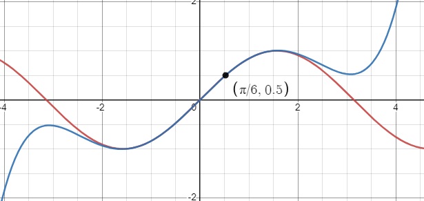
. This is a Taylor Polynomial. And it is the first two terms all the higher degree Taylor polynomial for f near x = a.

To fully understand these polynomials, there is a fair amount of preliminary stuff you need to understand. First you study sequences – functions whose domains are whole numbers. Next comes infinite series. A series is written by adding the terms of a sequence. (Sequences and series may have a finite or infinite number of terms. There is not much to say about finite series; infinite sequences and infinite series are where the action is.) oThe terms 0f some sequences and series are numbers. Other series have powers of an independent variable; these are called power series.   

Some power series approximate (converge to) the related function everywhere (i. e. for all Real numbers). Others provide a good approximation only on an interval of finite length. The intervals where the approximation is good is called the interval of convergence. Convergence tests – theorems really – help you determine if a series converges. These in tern help you find the interval of convergence. More on this in my next post.

Depending on your textbook and your teacher, you may study these topics in this order: sequences, convergence test, series, Taylor and Maclaurin polynimials for approximations, and power series. Others may change the order. The path may be different, but the destination will be the same.


Course and Exam Description Unit 10, Sections 10.1, 10.2, 10.11, 10.13, 10.14, 10.15. This is a BC only topic.  

Why Polar Equations?

The Cartesian coordinate system, the one you’ve been using up to now, is not the only way to find your way around the plane. In the Cartesian system, every point has two coordinates representing its distance and direction from the y-axis and the x-axis.

In the polar coordinate system points are identified by an ordered pair \displaystyle \left( {r,\theta } \right) by giving the direct distance, r, to the pole (the origin) and the angle measured counterwise from the polar axis (the positive x-axis) to the line from the pole to the point. The independent variable is \displaystyle \theta and r is a function of \displaystyle \theta .

Here is a Desmos program that will help you see how polar graphing works. Polar graphing paper shows concentric circles measuring the distance from the pole and with rays at common angles to help you locate points.

While there is a lot to be learned by studying polar curves¸ the AP Calculus BC exams are chiefly concerned with finding the area enclosed by a polar curve or between two polar curves, and the rates of change associated with a point moving along a polar curve. You will not be asked to name or know the equations of various curves (other than circles). The graphs are usually given, and your graphing calculator has a way of entering polar equations. (Be sure you learn how to do this.)

It has advantages in that some curves are much easier to write and graph in polar form than in Cartesian. In civil engineering (land surveying) it is easier to measure in the field an angle and a distance, rather than two right angles and two distances.

Changing back and forth from polar to Cartesian form is not difficult and you will learn a few formulas to accomplish this.

The polar coordinates of a point are not unique. The angle may be measured more than once around. This can be both an advantage and a disadvantage.


Course and Exam Description Unit 9, Sections 9.7 to 9.9. This is a BC only topic.

Why Parametric and Vector-Valued Functions?

Parametric and vector-valued functions are a way of writing and graphing more complicated, and therefore more interesting, curves.

Up to now you have been studying functions where the y-coordinates are found evaluating an expression in terms of the x-coordinates. Parametric and vector equations define both the x– and y-coordinates of a curve in terms of a third variable called a parameter, usually represented by t.

The only difference between the parametric and vector representation is the notation. The parametric form gives two equations, one for x and one for y. For example:

\displaystyle x\left( t \right)=t-1.2\sin (t)

\displaystyle y(t)=1-1.2\cos \left( t \right)

are the parametric equations of a curve called a prolate cycloid. It is the path of a point on the flange of a train wheel as it rolls along a straight track.

The vector form for this same curve is written:

\displaystyle \left\langle {t-1.2\sin \left( t \right),1-1.2\cos \left( t \right)} \right\rangle .

Notice the two coordinates of the vector are the same as the parametric equations.

In BC calculus you will study parametric and vector-valued equations of motion, that is the path of a point moving according to the parametric and vector equation. Since things are moving, they have a velocity – a vector pulling the point in the direction it is moving at any instant. The velocity vector is tangent to the curve and its length is the speed at which the point is moving.  Also, they have an acceleration – a vector pulling the velocity vector. These are found, as I hope you suspect, by differentiating. Vector-valued functions may also be integrated.

The illustration shows the path of a point on the flange of a train wheel rolling along a track. Notice that sometimes the point is moving backwards! The Position vector (from the origin to the point) is in black. Its endpoint is the point defined by the parametric or vector equations. The red vector is the velocity vector “pulling” the point to its next position. The green vector is the acceleration vector “pulling” the velocity vector.

While there are many other uses for parametric and vector-valued functions, the BC Calculus Exam only considers motion situations.


Course and Exam Description Unit 9, Sections 9.1 to 9.6. This is a BC only topic.

Why Applications?

I guess the obvious answer is so you will have something to use your new knowledge of the definite integral on. This unit is a collection of the first applications. There are many more.

The whole idea is based on the fact that a definite integral is a sum. Thus, they can be used to add things. Complicated shapes can be divided into simple shapes, like rectangles, and their areas can be added.

Here are the first uses.

AVERAGE VALUE OF A FUNCTION ON AN INTERVAL

You know that to average two numbers you add them and divide the total by two. To average a larger set of numbers you add them and divide the sum by the number of numbers. Now you will learn how to average the infinite number of y-values of a function over an interval. To do it you use a definite integral.

HINT: Average value of a function, average rate of change of a function, and the mean value theorem all sound kind of the same. Furthermore, the formulas all look kind of the same. Don’t mix them up. Use their full name, not just “average,” and use the right one.

There is an interesting result found some years ago by a tenth-grade student who took AB Calculus in eighth grade and BC in ninth. He proved that Most Triangles Are Obtuse! using the average value integral.

LINEAR MOTION

This application extends your previous work on objects moving on a line. By adding, with a definite integral, you will be able to determine how far the object moves in a given time. Knowing that and where the object starts, you will be able to find its current position. BC students will also learn how to find the length of a curve in the plane.

THE AREA BETWEEN TWO CURVES

This application extends what you know about finding the area between a curve and the x-axis to finding the area between two curves.

VOLUME OF A SOLID FIGURE WITH A REGULAR CROSS-SECTION

Some solid objects, when sliced in the right way, have regular cross-section. That means, the cut surface is a square, a rectangle, a right triangle, a semi-circle and so on. Think of cutting a piece of butter from a stick of butter – each piece is a square with a little thickness, like a very small pizza box. By using an integral to add their volumes you can find the volume of the original figure. .

VOLUME OF A SOLID OF REVOLUTION – DISK METHOD

A region in the plane is revolved aroud a line resulting in a solid figure. Finding its volume is just a special case of a solid with regular cross section where the cross section is a circle. Each little piece is a disk. By adding their volumes with an integral you can calculate the volume.

VOLUME OF A SOLID OF REVOLUTION – WASHER METHOD

Some solids of revolution have holes through them. These are formed by revolving a plane figure (usually the region between two curves) around an edge or a line outside the figure. The line is often the x– or y-axis. There is a formula for doing this, but understanding what you are doing – doing two disk problems – will help you with doing this. (See Subtract the Hole from the Whole.)

One last hint: You will want to know what the solid figure looks like. In addition to the illustrations in your textbook, there are various places online where you can find pictures of the figures. You can build models of them. There is an excellent iPad app called A Little Calculus that does a good job of illustrating and animating solid figures (and lots of other calculus stuff).

Course and Exam Description Unit 8