The Logistic Equation

After my last post, I realized I have never written about the logistic growth model. This is a topic tested on the AP Calculus BC exam (and not on AB). Here is a brief outline of this topic.

Logistic growth occurs in situations where the rate of change of a population, y, is proportional to the product of the number present at any time, y¸ and the difference between the number present and a number, C > 0, called the carrying capacity.

As explained in my last post, some factor limits the overall population possible to an amount C. Ask your students to sketch what they think the graph of such a function may look like and explain why.

The population starts by growing rapidly and then slows down as it approaches C. For example, if a small population of rabbits is placed on an island, the population will grow rapidly until the food starts to run out. The population will eventually level off and not grow greater than there is food to support it.

In symbols, logistic growth is modeled by the differential equation

$\displaystyle \frac{dy}{dt}=ky\left( C-y \right)$ , where k > 0 is the constant of proportionality, or by

$\displaystyle \frac{dy}{dt}=Ky\left( 1-\frac{y}{C} \right)$ and $K=Ck$

The differential equation is solved using separation of variables followed by using the method of partial fraction to obtain two expressions that can be integrated. The actual solving of the differential equation has never been tested, nor has memorization of the solution. What has been tested is what the solution graph looks like and how those features apply in real situations.

The solution, which need NOT be memorized, is $\displaystyle f\left( x \right)=\frac{C{{e}^{kCx}}}{{{e}^{kCx}}+kcD}$ (D is the constant of integration formally known as “+C.”)

The important features of the graph of the function can be found by examining the differential equation. This is an exercise consistent with MPAC 4: Connecting multiple representations and MPAC 5: Building notational fluency.

The figure above shows the slope field for a typical logistic differential equation. The values of y where $\frac{dy}{dt}=0$ indicate the location of a horizontal asymptote. There are horizontal asymptotes at y = 0 and y = C.

For points between the asymptotes $0<y<C$ , all the factors of the differential equation are positive. This indicates that the function is increasing. Near y = 0 and y = C one factor or the other is small, approaching 0: the graph of the solution (heavy blue line) is leveling off and approaching y = C from below as an asymptote. If the graph is extended into the second quadrant (thin blue line), it approaches the x-axis from above as an asymptote.

If the initial condition is greater than C then the (C – y) factor is negative, and the solution function is decreasing and approaching the asymptote y = C from above. If the number of rabbits put on the island is more than the carrying capacity, the population decreases (the poor rabbits starve).

The differential equation is a quadratic in y. Moving from the initial condition to right the slope of the tangent lines are positive and increasing, so the solution’s graph is concave upwards. After $y=\tfrac{1}{2}C$ the values of the slope (differential equation) remain positive but decrease indicating that the graph is now increasing and concave down. After this point the two factors of the differential equation switch values; that is, moving the same distance left and right of this point the product will be the same, but the values of each factor will have switched. Thus, the point where $y=\tfrac{1}{2}C$ is not only a point of inflection, but also a point of symmetry of the graph.

The maximum value occurs of the first derivative (the differential equation) is at $y=\tfrac{1}{2}C$ . This can be determined from the properties of a quadratic expression or from the second derivative,

$\displaystyle \frac{{{d}^{2}}y}{d{{t}^{2}}}=k\left( y\left( -1 \right)+\left( C-y \right)\left( 1 \right) \right)\cdot \frac{dy}{dt}=k\left( C-2y \right)\frac{dy}{dt}$ .

The second derivative is 0 at $y=\tfrac{1}{2}C$ . This is a point of inflection, the place where the function is increasing most rapidly.

Here is a Desmos demonstration that can be used to investigate the logistic differential equation, its slope field, and solution.

These ideas have all been tested on various BC exams. I cannot quote the questions here, but you may look them up for yourself.

Free-response:

2004 BC 5: (a) asymptotes as limits, and (b) when is the population growing fastest.

2008 BC 6: (a) sketch logistic equation on given slope field for two initial conditions – one between the asymptotes and one above the carrying capacity

Multiple-choice:

2003 BC 21: asymptote as a limit

2008 AB 22: Even though not an AB topic, the translation from words to symbols of the logistic model was tested on the 2008 AB multiple-choice exam. The idea was the translating, not knowledge of the logistic model.

2008 BC 24 given graph, identify differential equation.

2012 BC 14 identify logistic differential equation

There are also logistic questions on the restricted multiple-choice BC exams from 2013, 2014, and 2016; you’ll have to find them for yourself.

If you would like to experiment with logistic equations try graphing using Winplot for PC, Winplot for MACs, Geogebra, or some other program that will graph slope fields and solutions and has sliders. Desmos does not currently graph slope fields, but the solution graph can be produced.

For the differential equation enter 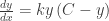$\frac{dy}{dx}=ky\left( C-y \right)$ with sliders for k and C.

If you just want to look at the solution, use any grapher with sliders. The solution can be graphed as $\displaystyle f\left( x \right)=\frac{C{{e}^{kCx}}}{{{e}^{kCx}}+kcD}$ with D, the constant of integration, added as a third slider.

Revised and Desmos Demo link added May 12, 2022

4 thoughts on “The Logistic Equation”

Brandon Kelly on July 30, 2020 at 18:35 said:

This is my first year teaching BC after 10 years of teaching AB. I’m looking at material left by last years BC teacher and they taught homogeneous differentials. Is that on the BC test?

LikeLike

Reply ↓
- Lin McMullin on August 2, 2020 at 09:23 said:
  
  No, only separable differentials are now tested. homogeneous differential equations were tested in BC before 1988.
  
  check the 2019 Course and Exam Description for what is currently required and tested.
  
  LikeLike
  
  Reply ↓
fangirllikehell on March 15, 2018 at 21:39 said:

THANK YOU

LikeLike

Reply ↓
Pingback: AP Calculus BC Cram Sheet - Magoosh High School Blog