Interpreting Graphs

Posted on February 27, 2013 by Lin McMullin

AP Type Questions 1

The long name is “Here’s the graph of the derivative, tell me things about the function.”

Most often students are given the graph identified as the derivative of a function. There is no equation given and it is not expected that students will write the equation (although this may be possible); rather, students are expected to determine important features of the function directly from the graph of the derivative. They may be asked for the location of extreme values, intervals where the function is increasing or decreasing, concavity, etc. They may be asked for function values at points.

The graph may be given in context and student will be asked about that context. The graph may be identified as the velocity of a moving object and questions will be asked about the motion and position. (Motion problems will be discussed as a separate type in a later post.)

Less often the function’s graph may be given and students will be asked about its derivatives.

What students should be able to do:

Read information about the function from the graph of the derivative. This may be approached as a derivative techniques or antiderivative techniques.
Find where the function is increasing or decreasing.
Find and justify extreme values (1^st and 2^nd derivative tests, Closed interval test, aka. Candidates’ test).
Find and justify points of inflection.
Find slopes (second derivatives, acceleration) from the graph.
Write an equation of a tangent line.
Evaluate Riemann sums from geometry of the graph only.
FTC: Evaluate integral from the area of regions on the graph.
FTC: The function, g(x), maybe defined by an integral where the given graph is the graph of the integrand, f(t), so students should know that if, $\displaystyle g\left( x \right)=g\left( a \right)+\int_{a}^{t}{f\left( t \right)dt}$ then ${g}'\left( x \right)=f\left( x \right)$ and ${{g}'}'\left( x \right)={f}'\left( x \right)$ .

The ideas and concepts that can be tested with this type question are numerous. The type appears on the multiple-choice exams as well as the free-response. They have accounted for almost 25% of the points available on recent test. It is very important that students are familiar with all of the ins and outs of this situation.

As with other questions, the topics tested come from the entire year’s work, not just a single unit. In my opinion many textbooks do not do a good job with these topics.

Study past exams; look them over and see the different things that can be asked.

For some previous posts on this subject see October 15, 17, 19, 24, 26, 2012 January 25, 28, 2013

The AP Calculus Exams

Posted on February 25, 2013 by Lin McMullin

I assume that most of my readers are AP Calculus teachers. The year is coming to an end and it is time to think about reviewing for the exams. For the next few weeks my posts will discuss how to review for the AP calculus exams. Don’t panic if you’re not done yet; it’s too early for that. I am just trying to stay ahead of you so you’ll be able to think this over before its time to use it.

The first post will be some general information about the exam for your students. After that there will be a series of post on each of the “type” problems that appear on the free-response sections exams. A good way to review is to spend 2 – 3 days on each type so that students can see what and how each topic is tested. Doing so will help them not only with the free-response questions, but also with the multiple-choice questions which test the same concepts in bits and pieces.

I would like you to share your ideas as well. Please respond by clicking on “Comments” at the end of each post with your suggestions. You can also find what I’ve written about specific topics by using the search box or the categories list in the right-side column, or by clicking on any of the words in the tag cloud at the bottom of the page. This will bring up all the post about that topic.

Ideas for Reviewing for the AP Exams

Posted on February 25, 2013 by Lin McMullin

Part of the purpose of reviewing for the AP calculus exams is to refresh your students’ memory on all the great things you’ve taught them during the year. The other purpose is to inform them about the format of the exam, the style of the questions, the way they should present their answer and how the exam is graded and scored.

Using AP questions all year is a good way to accomplish some of this. Look through the released multiple-choice exam and pick questions related to whatever you are doing at the moment. Free-response questions are a little trickier since the parts of the questions come from different units. These may be adapted or used in part.

At the end of the year, I suggest you review the free-response questions by type – table questions, differential equations, area/volume, rate/accumulation, graph, etc. That is, plan to spend a few days doing a selection of questions of one type so that student can see how the way that type question can be used to test a variety of topics. Then go onto the next type. Many teachers keep a collection of past free-response questions filed by type rather than year. This makes it easy to study them by type.

In the next few posts I will discuss each type in turn and give suggestions about what to look for and how to approach the question.

Simulated Exam

Plan to give a simulated exam. Each year the College Board makes a full exam available. The exams for 1998, 2003, 2008 are available at AP Central and the 2012 and the 2013 exams are available through your audit website. If possible find a time when your students can take the exam in 3.25 hours. Teachers often do this on a weekend. This will give your students a feel for what it is like to work calculus problems under test conditions. If you cannot get 3.25 hours to do this give the sections in class using the prescribed time. Some teachers schedule several simulated exam. Of course you need to correct them and go over the most common mistakes.

Explain the scoring

There are 108 points available on the exam; each half is worth the same – 54 points. The number of points required for each score is set after the exams are graded.

For the AB exam the points required for each score out of 108 point are, very approximately:

for a 5 – 69 points,
for a 4 – 52 points,
for a 3 – 40 points,
for a 2 – 28 points.

The numbers are similar for the BC exams are again very approximately:

for a 5 – 68 points,
for a 4 – 58 points,
for a 3 – 42 points,
for a 2 – 34 points.

The actual numbers are not what is important. What is important is that students can omit or get wrong a large number of questions and still get a good score. Students may not be used to this (since they skip or get wrong so few questions on your tests). They should not panic or feel they are doing poorly if they miss a number of questions. If they understand and accept this in advance they will calm down and do better on the exams. Help them understand they should gather as many points as they can, and not be too concerned if the cannot get them all. Doing only the first 2 parts of a free-response question will probably put them at the mean for that question. Remind them not to spend time on something that’s not working out, or that they don’t feel they know how to do.

Resources

Here are several resources that will help you get started:

“The AP Calculus Exam: How, not only to Survive, but to Prevail…” – Advice for students on the format of the exam and do’s and don’ts for the exam. Print this and share it with your students.
The AB Directions and BC Directions. Yes, this is boiler plate stuff, but take a few minutes to go over it with your students. They should not have to see the directions for the first time on the day of the exam. I have highlighted some of the more important directions
Calculator Skills – share this information with your students, if you have not already done so. There are only about 12 -15 points on the entire exam which require a calculator. A calculator alone will not get anyone a 5 (or even a 2). Nevertheless, the points are there and usually pretty easy to earn. The real reason calculators and other technology are so important is that when used throughout the year, they help students better understand the calculus.

The next post: The Graph Stem Question

Error Bounds

Posted on February 22, 2013 by Lin McMullin

How Good is Your Approximation?

Whenever you approximate something, you should be concerned about how good your approximation is. The error, E, of any approximation is defined to be the absolute value of the difference between the actual value and the approximation. If T_n(x) is the Taylor/Maclaurin approximation of degree n for a function f(x) then the error is $E=\left| f\left( x \right)-{{T}_{n}}\left( x \right) \right|$ . This post will discuss the two most common ways of getting a handle on the size of the error: the Alternating Series error bound, and the Lagrange error bound.

Both methods give you a number B that will assure you that the approximation of the function at $x={{x}_{0}}$ in the interval of convergence is within B units of the exact value. That is,

$\left( f\left( {{x}_{0}} \right)-B \right)<{{T}_{n}}\left( {{x}_{0}} \right)<\left( f\left( {{x}_{0}} \right)+B \right)$

${{T}_{n}}\left( {{x}_{0}} \right)\in \left( f\left( {{x}_{0}} \right)-B,\ f\left( {{x}_{0}} \right)+B \right)$ .

Stop for a moment and consider what that means: $f\left( {{x}_{0}} \right)-B$ and $f\left( {{x}_{0}} \right)+B$ are the endpoints of an interval around the actual value and the approximation will lie in this interval. Ideally, B is a small (positive) number.

Alternating Series

If a series $\sum\limits_{n=1}^{\infty }{{{a}_{n}}}$ alternates signs, decreases in absolute value and $\underset{n\to \infty }{\mathop{\lim }}\,\left| {{a}_{n}} \right|=0$ then the series will converge. The terms of the partial sums of the series will jump back and forth around the value to which the series converges. That is, if one partial sum is larger than the value, the next will be smaller, and the next larger, etc. The error is the difference between any partial sum and the limiting value, but by adding an additional term the next partial sum will go past the actual value. Thus, for a series that meets the conditions of the alternating series test the error is less than the absolute value of the first omitted term:

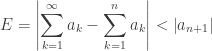
$\displaystyle E=\left| \sum\limits_{k=1}^{\infty }{{{a}_{k}}}-\sum\limits_{k=1}^{n}{{{a}_{k}}} \right|<\left| {{a}_{n+1}} \right|$ .

Example: $\sin (0.2)\approx (0.2)-\frac{{{(0.2)}^{3}}}{3!}=0.1986666667$ The absolute value of the first omitted term is $\left| \frac{{{(0.2)}^{5}}}{5!} \right|=0.26666\bar{6}\times {{10}^{-6}}$ . So our estimate should be between $\sin (0.2)\pm 0.266666\times {{10}^{-6}}$ (that is, between 0.1986666641 and 0.1986719975), which it is. Of course, working with more complicated series, we usually do not know what the actual value is (or we wouldn’t be approximating). So an error bound like $0.26666\bar{6}\times {{10}^{-6}}$ assures us that our estimate is correct to at least 5 decimal places.

The Lagrange Error Bound

Taylor’s Theorem: If f is a function with derivatives through order n + 1 on an interval I containing a, then, for each x in I , there exists a number c between x and a such that

$\displaystyle f\left( x \right)=\sum\limits_{k=1}^{n}{\frac{{{f}^{\left( k \right)}}\left( a \right)}{k!}{{\left( x-a \right)}^{k}}}+\frac{{{f}^{\left( n+1 \right)}}\left( c \right)}{\left( n+1 \right)!}{{\left( x-a \right)}^{n+1}}$

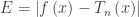
The number $\displaystyle R=\frac{{{f}^{\left( n+1 \right)}}\left( c \right)}{\left( n+1 \right)!}{{\left( x-a \right)}^{n+1}}$ is called the remainder.

The equation above says that if you can find the correct c the function is exactly equal to T_n(x) + R. Notice the form of the remainder is the same as the other terms, except it is evaluated at the mysterious c. The trouble is we almost never can find the c without knowing the exact value of f(x), but; if we knew that, there would be no need to approximate. However, often without knowing the exact values of c, we can still approximate the value of the remainder and thereby, know how close the polynomial T_n(x) approximates the value of f(x) for values in x in the interval, i.

Corollary – Lagrange Error Bound.

$\displaystyle \left| \frac{{{f}^{\left( n+1 \right)}}\left( c \right)}{\left( n+1 \right)!}{{\left( x-a \right)}^{n+1}} \right|\le \left( \text{max}\left| {{f}^{\left( n+1 \right)}}\left( x \right) \right| \right)\frac{{{\left| x-a \right|}^{n+1}}}{\left( n+1 \right)!}$

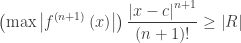
The number $\displaystyle \left( \text{max}\left| {{f}^{\left( n+1 \right)}}\left( x \right) \right| \right)\frac{{{\left| x-c \right|}^{n+1}}}{\left( n+1 \right)!}\ge \left| R \right|$ is called the Lagrange Error Bound. The expression $\left( \text{max}\left| {{f}^{\left( n+1 \right)}}\left( x \right) \right| \right)$ means the maximum absolute value of the (n + 1) derivative on the interval between the value of x and c. The corollary says that this number is larger than the amount we need to add (or subtract) from our estimate to make it exact. This is the bound on the error. It requires us to, in effect, substitute the maximum value of the n + 1 derivative on the interval from a to x for ${{f}^{(n+1)}}\left( x \right)$ . This will give us a number equal to or larger than the remainder and hence a bound on the error.

Example: Using the same example sin(0.2) with 2 terms. The fifth derivative of $\sin (x)$ is $-\cos (x)$ so the Lagrange error bound is $\displaystyle \left| -\cos (0.2) \right|\frac{\left| {{\left( 0.2-0 \right)}^{5}} \right|}{5!}$ , but if we know the cos(0.2) there are a lot easier ways to find the sine. This is a common problem, so we will pretend we don’t know cos(0.2), but whatever it is its absolute value is no more than 1. So the number $\left( 1 \right)\frac{\left| {{\left( 0.2-0 \right)}^{5}} \right|}{5!}=2.6666\bar{6}\times {{10}^{-6}}$ will be larger than the Lagrange error bound, and our estimate will be correct to at least 5 decimal places.

This “trick” is fairly common. If we cannot find the number we need, we can use a value that gives us a larger number and still get a good handle on the error in our approximation.

FYI: $\displaystyle \left| -\cos (0.2) \right|\frac{\left| {{\left( 0.2-0 \right)}^{5}} \right|}{5!}\approx 2.61351\times {{10}^{-6}}$

Corrected: February 3, 2015, June 17, 2022

New Series from Old 3

Posted on February 20, 2013 by Lin McMullin

Rational Functions and a “mistake”

A geometric series is one in which each term is found by multiplying the preceding term by the same number or expression. This number is called the common ratio, r. Geometric series converge if, and only if, $\left| r \right|<1$ . If a geometric series converges, then the sum of the (infinite number of) terms is $\displaystyle \frac{{{a}_{1}}}{1-r}$ where a₁ is the first term.

We can use this to write series for rational expressions.

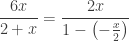
Example 1. The series for $\displaystyle \frac{1}{1+{{x}^{2}}}$ that we assumed in the last post can be rewritten as $\displaystyle \frac{1}{1-\left( -{{x}^{2}} \right)}$ . This has the same form as the sum of the geometric series so we can write it as a geometric series with a₁ = 1 and r = –x² . The result is

$\displaystyle \frac{1}{1+{{x}^{2}}}=1-{{x}^{2}}+{{x}^{4}}-{{x}^{6}}+\cdots +{{\left( -1 \right)}^{2n-1}}{{x}^{2n-2}}+\cdots ,\quad -1<x<1$

Example 2: $\displaystyle \frac{6x}{2+x}=\frac{2x}{1-\left( -\tfrac{x}{2} \right)}$ . Letting ${{a}_{1}}=3x$ and $r=-\tfrac{x}{2}$ we have

$\displaystyle \frac{6x}{2+x}=\frac{3x}{1-\left( -\tfrac{x}{2} \right)}=3x+3x\left( -\tfrac{x}{2} \right)+3x{{\left( -\tfrac{x}{2} \right)}^{2}}+3x{{\left( -\tfrac{x}{2} \right)}^{3}}+\cdots$

$\displaystyle \frac{6x}{2+x}=3x-\tfrac{3}{2}{{x}^{2}}+\tfrac{3}{4}{{x}^{3}}-\tfrac{3}{8}{{x}^{4}}+\tfrac{3}{16}{{x}^{5}}+\cdots +\tfrac{{{\left( -1 \right)}^{2n-1}}}{{{2}^{n-1}}}3{{x}^{n}}+\cdots$

The interval of convergence is $\left| -\tfrac{x}{2} \right|<1$ or $-2<x<2$ .

Many power series for rational functions can be obtained in this way.

An instructive “mistake.”

I have heard of students making an interesting mistake with this kind of problem. Instead of dividing by 2, they divide by x and arrive at $\displaystyle \frac{6x}{2+x}=\frac{6}{1-\left( -\tfrac{2}{x} \right)}$ and then write the series as

$\displaystyle \frac{6x}{2+x}=\frac{6}{1-\left( -\tfrac{2}{x} \right)}=6+6\left( -\tfrac{2}{x} \right)+6{{\left( -\tfrac{2}{x} \right)}^{2}}+6{{\left( -\tfrac{2}{x} \right)}^{3}}+\cdots$

$\displaystyle \frac{6x}{2+x}=6-\frac{12}{x}+\frac{24}{{{x}^{2}}}-\frac{48}{{{x}^{3}}}+\frac{96}{{{x}^{4}}}-\cdots$

With an interval of convergence of $\left| -\tfrac{2}{x} \right|<1$ or $x<-2\text{ or }x>2$ . Now this is not a Taylor series since the powers are in the denominators, but it is nevertheless interesting. Let’s look at the graphs.

The rational expression is the black graph and partly hidden by the other graphs where they converge. The blue graph is the 5^th degree Taylor Polynomial and its interval of convergence is the white strip in the center of the graph. The red graph is the “mistake” (also 5th degree) with the two blue regions as its interval of convergence. Both series fit the rational function but only in their own interval of convergence.

New Series from Old 2

Posted on February 18, 2013 by Lin McMullin

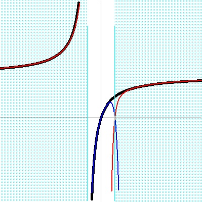
Differentiating and integrating a known series can help you find other series. Since $\frac{d}{dx}\sin \left( x \right)=\cos \left( x \right)$ we can find the series for cos(x) this way

$\frac{d}{dx}\sin \left( x \right)=\frac{d}{dx}(x-\frac{{{x}^{3}}}{3!}+\frac{{{x}^{5}}}{5!}-\frac{{{x}^{7}}}{7!}+\cdots +\frac{{{\left( -1 \right)}^{n-1}}{{x}^{2n-1}}}{\left( 2n-1 \right)!}+\cdots )$

$\frac{d}{dx}\sin \left( x \right)=1-\frac{3{{x}^{2}}}{3!}+\frac{5{{x}^{4}}}{5!}-\frac{7{{x}^{6}}}{7!}+\cdots \frac{{{\left( -1 \right)}^{n-1}}\left( 2n-1 \right){{x}^{2n}}}{\left( 2n-1 \right)!}+\cdots$

$\cos \left( x \right)=1-\frac{{{x}^{2}}}{2!}+\frac{{{x}^{4}}}{4!}-\frac{{{x}^{6}}}{6!}+\cdots \frac{{{\left( -1 \right)}^{n-1}}{{x}^{2n}}}{\left( 2n \right)!}+\cdots$

Of course, we could also have integrated the series for sin(x) to get the series for –cos(x) and then changed the signs.

In our next post we will find that

$\frac{1}{1+{{x}^{2}}}=1-{{x}^{2}}+{{x}^{4}}-{{x}^{6}}+\cdots +{{\left( -1 \right)}^{2n+1}}{{x}^{2n-2}}+\cdots$

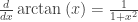
Recall that $\frac{d}{dx}\arctan \left( x \right)=\frac{1}{1+{{x}^{2}}}$ , so we can integrate the series above to find the series for arctan(x).

$\arctan \left( x \right)=\int_{{}}^{{}}{(1-{{x}^{2}}+{{x}^{4}}-{{x}^{6}}+\cdots +{{\left( -1 \right)}^{2n-1}}{{x}^{2n-2}}+\cdots )dx}$

$\arctan \left( x \right)=C+x-\tfrac{1}{3}{{x}^{3}}+\tfrac{1}{5}{{x}^{5}}-\tfrac{1}{7}{{x}^{7}}+\cdots +\tfrac{{{\left( -1 \right)}^{2n+1}}}{2n-1}{{x}^{2n-1}}+\cdots$

Since $\arctan \left( 0 \right)=0$ it follows that the constant of integration $C=0$ so

$\arctan \left( x \right)=x-\tfrac{1}{3}{{x}^{3}}+\tfrac{1}{5}{{x}^{5}}-\tfrac{1}{7}{{x}^{7}}+\cdots +\tfrac{{{\left( -1 \right)}^{2n+1}}}{2n-1}{{x}^{2n-1}}+\cdots$

When differentiating or integrating the interval of convergence cannot get any larger, but it can get smaller. If the endpoints are included before differentiating or integrating then you must check to see if they are included in the new series.

Next post: Rational functions and geometric series.

New Series from Old 1

Posted on February 15, 2013 by Lin McMullin

There are three common ways to get new series from old series without calculating all the derivatives and substituting into the Taylor Series general term.

Substituting into known series
Differentiating and integrating
Approaching rational functions as geometric series

This will be the subject of this and my next two posts.

Substituting

As you might expect the Taylor/Maclaurin series for the “parent” functions are known. We’ve seen the series for ln(x) and sin(x) and you can develop or look up series for e^x, cos(x) and so on. The power series for compositions involving these series can be found by substituting.

Example 1: To find the Maclaurin series for sin(3x), substitute 3x for x in the sin(x) series

$\sin (x)=x-\frac{{{x}^{3}}}{3!}+\frac{{{x}^{5}}}{5!}-\frac{{{x}^{7}}}{7!}+\cdots +\frac{{{\left( -1 \right)}^{n-1}}{{x}^{2n-1}}}{\left( 2n-1 \right)!}+\cdots$

$\sin (3x)=\left( 3x \right)-\frac{{{\left( 3x \right)}^{3}}}{3!}+\frac{{{\left( 3x \right)}^{5}}}{5!}-\frac{{{\left( 3x \right)}^{7}}}{7!}+\cdots +\frac{{{\left( -1 \right)}^{n-1}}{{\left( 3x \right)}^{2n-1}}}{\left( 2n-1 \right)!}+\cdots$

Substituting along with some algebra also works, as the next example shows.

Example 2: To find the series for multiply the last answer by x²

${{x}^{2}}\sin (3x)=\left( 3x \right){{x}^{2}}-\frac{{{\left( 3x \right)}^{3}}{{x}^{2}}}{3!}+\frac{{{\left( 3x \right)}^{5}}{{x}^{2}}}{5!}-\cdots +\frac{{{\left( -1 \right)}^{n-1}}{{\left( 3x \right)}^{2n-1}}{{x}^{2}}}{\left( 2n-1 \right)!}+\cdots$

${{x}^{2}}\sin (3x)=3{{x}^{3}}-\frac{{{3}^{3}}{{x}^{5}}}{3!}+\frac{{{3}^{5}}{{x}^{7}}}{5!}-\cdots +\frac{{{\left( -1 \right)}^{n-1}}{{3}^{2n-1}}{{x}^{2n+1}}}{\left( 2n-1 \right)!}+\cdots$

Example 3: You must be a little careful sometimes. A recent AP Calculus exam asked for the first 4 terms of the Maclaurin series for $\sin \left( 5x+\tfrac{\pi }{4} \right)$ . Substituting $\sin \left( 5x+\tfrac{\pi }{4} \right)$ into the sin(x) series gives a series centered at $x=-\tfrac{\pi }{20}$ but the questions required a series centered at x = 0. Almost all students calculated derivatives and used them in the general form of a Maclaurin series. But with a little trigonometry you can substitute after some rewriting:

$\sin \left( 5x+\tfrac{\pi }{4} \right)=\sin \left( 5x \right)\cos \left( \tfrac{\pi }{4} \right)+\cos \left( 5x \right)\sin \left( \tfrac{\pi }{4} \right)$

$\sin \left( 5x+\tfrac{\pi }{4} \right)=\tfrac{\sqrt{2}}{2}\left( \sin \left( 5x \right)+\cos \left( 5x \right) \right)$

Now we can substitute into the series for the sin(x) and cos(x):

$\sin \left( 5x+\tfrac{\pi }{4} \right)=\tfrac{\sqrt{2}}{2}\left( \left( 5x-\frac{{{\left( 5x \right)}^{3}}}{3!} \right)+\left( 1-\frac{{{\left( 5x \right)}^{2}}}{2!} \right) \right)$

$\sin \left( 5x+\tfrac{\pi }{4} \right)=\tfrac{\sqrt{2}}{2}+\tfrac{5\sqrt{2}}{2}x-\tfrac{25\sqrt{2}}{4}{{x}^{2}}-\tfrac{125\sqrt{2}}{12}{{x}^{3}}$

As you can see from the last two examples, any sort of “legal” algebra or trigonometry can be used to find a new series from one you already know.

Next post: Differentiating and Integrating

Teaching Calculus

The pleasure lies not in discovering the truth, but in searching for it.

Monthly Archives: February 2013

Interpreting Graphs

The AP Calculus Exams

Ideas for Reviewing for the AP Exams

Error Bounds

New Series from Old 3

New Series from Old 2

New Series from Old 1

Share this:

Share this:

Share this:

Share this:

Share this:

Share this:

Share this: