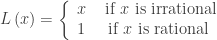
This is a re-post and update of the first in a series of posts from last year. It contains links to posts on this blog about the topics of limits and continuity for your reference in planning. Other updated post on the 2019 CED will come throughout the year, hopefully, a few weeks before you get to the topic.
Unit 1 contains topics on Limits and Continuity. (CED – 2019 p. 36 – 50). These topics account for about 10 – 12% of questions on the AB exam and 4 – 7% of the BC questions.
Logically, limits come before continuity since limit is used to define continuity. Practically and historically, continuity comes first. Newton and Leibnitz did not have the concept of limit the way we use it today. It was in the early 1800’s that the epsilon-delta definition of limit was first given by Bolzano (whose work was overlooked) and then by Cauchy, Jordan, and Weierstrass. But, their formulation did not use the word “limit”, rather the use was part of their definition of continuity. Only later was it pulled out as a separate concept and then returned to the definition of continuity as a previously defined term. See Which Came First?
Students should have plenty of experience in their math courses before calculus with functions that are and are not continuous. They should know the names of the types of discontinuities – jump, removable, infinite, oscillating etc.and the related terms such as asymptote. As you go through this unit, you may want to quickly review these terms and concepts as they come up.
(As a general technique, rather than starting the year with a week or three of review – which the students need but will immediately forget again – be ready to review topics as they come up during the year as they are needed – you will have to do that anyway. See Getting Started #2)
Topics 1.1 – 1.9: Limits
Topic 1.1: Suggests an introduction to calculus to give students a hint of what’s coming. See Getting Started #3
Topic 21.: Proper notation and multiple-representations of limits.
There is an exclusion statement noting that the delta-epsilon definition of limit is not tested on the exams, but you may include it if you wish. The epsilon-delta definition is not tested probably because it is too difficult to write good questions. Specifically, (1) the relationship for a linear function is always  where m is the slope and is too complicated to compute for other functions, and (2) for a multiple-choice question the smallest answer must be correct. (Why?)
Topic 1.3: One-sided limits.
Topic 1.4: Estimating limits numerically and from tables.
Topic 1.5: Algebraic properties of limits.
Topic 1.6: Simplifying expressions to find their limits. This can and should be done along with learning the other concepts and procedures in this unit.
Topic 1.7: Selecting the proper procedure for finding a limit. The first step is always to substitute the value into the limit. If this comes out to be number than that is the limit. If not, then some manipulation may be required. This can and should be done along with learning the other concepts and procedures in this unit.
Topic 1.8: The Squeeze Theorem is mainly used to determine  which in turn is used in finding the derivative of the sin(x). (See Why Radians?) Most of the other examples seem made up just for exercises and tests. (See 2019 AB 6(d)). Thus, important, but not too important.
Topic 1.9: Connecting multiple-representations of limit. This can and should be done along with learning the other concepts and procedures in this unit. Dominance, Topic 15, may be included here as well (EK LIM-2.D.5)
Topics 1.10 – 1.16 Continuity
Topic 1.10: Here you can review the different types of discontinuities with examples and graphs.
Topic 1.11: The definition of continuity. The EK statement does not seem to use the three-hypotheses definition. However, for the limit to exist and for f(c) to exist, they must be real numbers (i.e. not infinite). This is tested often on the exams, so students should have practice with verifying that (all three parts of) the hypothesis are met and including this in their answers.
Topic 1.12: Continuity on an interval and which Elementary Functions are continuous for all real numbers.
Topic 1.13: Removable discontinuities and handing piecewise – defined functions
Topic 1.14: Vertical asymptotes and unbounded functions. Here be sure to explain the difference between limits “equal to infinity” and limits that do not exist (DNE). See Good Question 5: 1998 AB2/BC2.
Topic 1.15: Limits at infinity, or end behavior of a function. Horizontal asymptotes are the graphical manifestation of limits at infinity or negative infinity. Dominance is included here as well (EK LIM-2.D.5)
Topic 1.16: The Intermediate Value Theorem (IVT) is a major and important result of a function being continuous. This is perhaps the first Existence Theorem students encounter, so be sure to stop and explain what an existence theorem is.
The suggested number of 40 – 50 minute class periods is 22 – 23 for AB and 13 – 14 for BC. This includes time for testing etc. If time seems to be a problem you can probably combine topics 3 – 5, topics 6 -7, topics 11 – 12. Topics 6, 7, and 9 are used with all the limit work.
There are three other important limits that will be coming in later Units:
The definition of the derivative in Unit 2, topics 1 and 2
L’Hospital’s Rule in Unit 4, topic 7
The definition of the definite integral in Unit 6, topic 3.
Posts on Continuity
CONTINUITY To help understand limits it is a good idea to look at functions that are not continuous. Historically and practically, continuity should come before limits. On the other hand, the definition of continuity requires knowing about limits. So, I list continuity first. The modern definition of limit was part of Weierstrass’ definition of continuity.
Which Came First? (7-28-2020)
Continuity (8-13-2012)
Continuity (8-21-2013) The definition of continuity.
Continuous Fun (10-13-2015) A fuller discussion of continuity and its definition
Right Answer – Wrong Question (9-4-2013) Is a function continuous even if it has a vertical asymptote?
Asymptotes (8-15-2012) The graphical manifestation of certain limits
Fun with Continuity (8-17-2012) the Diriclet function
Far Out! (10-31-2012) When the graph and dominance “disagree” From the Good Question series
Posts on Limits
Why Limits? (8-1-2012)
Deltas and Epsilons (8-3-2012) Why this topic is not tested on the AP Calculus Exams.
Finding Limits (8-4-2012) How to…
Dominance (8-8-2012) See limits at infinity
Determining the Indeterminate (12-6-2015) Investigating an indeterminate form from a differential equation. From the Good Question series.
Locally Linear L’Hôpital (5-31-2013) Demonstrating L’Hôpital’s Rule (a/k/a L’Hospital’s Rule)
L’Hôpital’s Rules the Graph (6-5-2013)
Here are links to the full list of posts discussing the ten units in the 2019 Course and Exam Description. the 2019 versions
2019 CED – Unit 1: Limits and Continuity
2019 CED – Unit 2: Differentiation: Definition and Fundamental Properties.
2019 CED – Unit 3: Differentiation: Composite , Implicit, and Inverse Functions
2019 CED – Unit 4 Contextual Applications of the Derivative Consider teaching Unit 5 before Unit 4
2019 – CED Unit 5 Analytical Applications of Differentiation Consider teaching Unit 5 before Unit 4
2019 – CED Unit 6 Integration and Accumulation of Change
2019 – CED Unit 7 Differential Equations Consider teaching after Unit 8
2019 – CED Unit 8 Applications of Integration Consider teaching after Unit 6, before Unit 7
2019 – CED Unit 9 Parametric Equations, Polar Coordinates, and Vector-Values Functions
2019 CED Unit 10 Infinite Sequences and Series


 .
. .
.
 . This function has a single hole in the graph at (3, 3); It one may be difficult to see. Try using ZDecimal. A single point is missing because there is no value at x= 3 because the denominator is zero.
 .
. Zoom in several times at (3, 0) where the function has no value.
 , is often used that way by those unlucky folks who don’t understand mathematics.
 . This fraction has no value when x = 3 because there the denominator is zero. And you cannot divide by zero. Nothing personal, no one, no matter how smart, can divide by zero. Ever. Permanently and forever not allowed. Don’t even think about it! (Actually, think about it; just don’t do it.)
 . This means that the expression gets larger as x gets closer to three. The expression will be greater than any (large) number you want, if you are close enough to three.
 . I say pick any value for x between 2.9999 and 3.0001 (
 ) and the expression will be larger than
  ? Try a number between 2.9999999999 and 3.0000000001. I can play this game all day.
 on your calculator. (Hint: Whenever you come across something like this, it is a great idea to graph the expression on your graphing calculator. Graphs can help you see what’s going on. Keep that in mind for the future.)
 .
.

 , sometimes called “negative infinity,” means that the expression gets less than (i.e. more negative), than any negative number you choose.
  has no value, is “undefined,” when x = 0, but
  . (Hint: this is where you should look at a graph on your graphing calculator to see why.)
 does not exist. This is very similar to the first example but look at the graph and you’ll see a big difference.
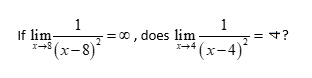


 , also known as
 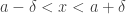 , will generate function values greater than M.
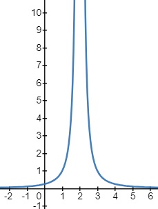

 will do the trick, since if


 . So, which is it “infinity” or does not exist”?
  does not exist and is not ∞ .
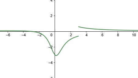
 has a finite jump discontinuity at x = 3.
  where m is the slope and is too complicated to compute for other functions, and (2) for a multiple-choice question the smallest answer must be correct. (Why?)
 which in turn is used in finding the derivative of the sin(x). (See
  if, and only if, (1)
  exists, (2)
  exists, and (3)
  .
. , if, and only if, for every number
  there exists a number
  such that if
  , then
  .
.