
Chip Rollinson is a teacher at Buckingham Browne & Nichols School in Cambridge, Massachusetts. Today’s post is a note he sent to the AP Calculus Community bulletin board that I found interesting. I will share it with you with his permission. I made some minor edits. Chip wrote on February 5, 2015:
I had an epiphany today about the relationship between Euler’s Method and compounding growth. I had never made the connection before. I thought it was cool so I decided I needed to share it.
Consider the differential equation 

Let’s look at this differential equation using Euler’s Method.

Leonhard Euler
1707 – 1783
Let’s start with a step size of 
After one step, you arrive at the point

After 2 steps, you arrive at the point

After 3 steps, you arrive at the point

After 4 steps, you arrive at the point

And so on …
After 12 steps, you arrive at the point

After 120 steps, you arrive at the point

After 12t steps, you arrive at the point
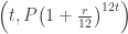
Do these y-values look familiar? It’s the amount you’d have if you were compounding monthly with a yearly interest rate of r for a year, 10 years, and t years.
If the step size were 

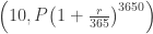

These y-values are the amount you’d have if you were compounding daily for a year, 10 years, and t years.
If the step size were 

If n went to infinity, you would arrive at the point 
I’d never made this connection before, but it makes perfect sense now.
The actual problem that got me thinking about all of this was:
Suppose that you now have $6000, you expect to save an additional $3000 during each year, and all of this is deposited in a bank paying 4% interest compounded continuously.
This generates the differential equation:

This was a fun one to do out. I started with a step size of 1/12 and then made them smaller. I derived the solution from Euler’s Method!
So writes Chip Rollinson. He included the following links to his computations: here and here
Then there were some interesting comments from others.
1. Mark Howell pointed out that if 
This would make a good exercise for your students to show given a derivative, a starting point, and a small number of steps. Try 


2. Dan Teague went further and pointed out that this is really the development of the Fundamental Theorem of Calculus for a particular function. He contributed this development of the concept.
So Thank You Chip for this and the several other comments you’ve contributed to other post on this blog. And thank you Mark and Dan for your contributions.
 ) from the initial point. The first step is exactly the local linear approximation idea.

 , is found by substituting the coordinates of the previous point into the differential equation. It has the form of the equation of a line.
 with the initial point (1, 3). Approximate the value of f(2) using Euler’s method with two steps of equal size.
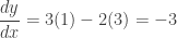 . Then
 and
and 
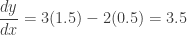
 and
and 
 . The exact value is 2.5545. A better approximation could be found using smaller steps.
 with the initial condition
  . The screen is two units wide extending from x = 0 to x = 2. The calculator graph below shows three graphs. The top graph is the particular solution
  . (I said it was easy.) The lower graph shows an approximate solution with the rather large step size of
  with the two points connected; look closely and you will see the two segments. The middle graph has a step size of
  . There are 8 segments, but they appear to be a smooth curve approximating the solution. Notice it is closer to the actual solution graph. An even smaller step size would show an even smoother graph closer to the particular solution.
